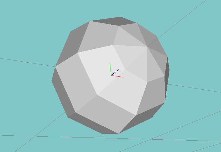
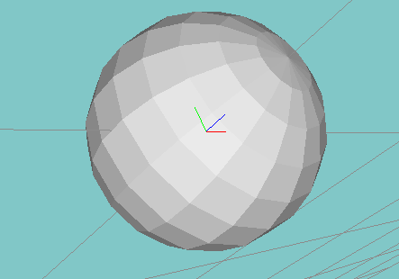
Coarse and fine spheres, above. The North and South poles of the spheres are aligned along
the Z axis.
Assignment 5 - Intro. to Geometry Processing
Due Wednesday Nov. 20, 2019 at 3:00 PM
Overview
In this assignment, you will implement a technique for smoothing meshes known as implicit fairing. The implementation requires you to build a variant of the discrete Laplacian as a matrix operator while utilizing the halfedge data structure to quickly traverse regions of a mesh for computations. The smoothing process ultimately occurs from solving a non-linear matrix equation that involves the discrete Laplacian operator and is of a similar form to a Poisson equation. You will set up the non-linear matrix equation using Eigen’s sparse matrix library and solve it using Eigen’s sparse solver. This will result in the smoothing of a given mesh, as shown with the Stanford bunny in the video above.
Before you begin, you may want to review the assignment material with these lecture notes. The files for this assignment can be downloaded here. More in-depth details for the assignment will be given in the sections below.
There is also an extra credit section at the bottom.
As something to keep in mind, the amount of coding for this assignment is quite small compared to that of previous assignments. However, the material this time around is arguably more difficult conceptually. Take the time to carefully read through the lecture notes and think out your algorithms before you start coding.
By the way, if you end up liking the material from this assignment a lot, then we highly recommend taking CS177 Discrete Differential Geometry taught by Prof. Peter Schröder. It is a great course that goes deep into the theory behind all these concepts that we merely glanced over. It is usually offered during the winter term.
Your Assignment
Your task is to write an OpenGL program in C++ that takes as input (1) one of the provided scene files, (2) integer and resolutions, and (3) a time step , and displays in the OpenGL window the smoothed mesh (computed via implicit fairing after the given time step).
The input of your program should be read from standard input as so:
To help guide you, we have broken the task of writing this program into parts.
The hard part here is that neither the .obj files for the bunny or armadillo have normal vectors this time around! (Make sure you can actually parse these files correctly!) You need to compute the normal vectors yourself using the halfedge data structure. We provide a simple halfedge implementation for you to use in the homework files. Alternatively, if you have your own halfedge library that you prefer, then feel free to use that instead. However, the TA’s ask that you do not use any libraries that require us to install a lot of dependencies.
Fill a halfedge data structure with data from your mesh. Then write a function that utilizes the convenience of the halfedge to compute the normal vectors per vertex. The lecture notes cover this a fair bit.
We recommend building off your Assignment 3 code. We don’t need GLSL at all for this assignment, though if you prefer Phong shading over Gouraud shading, then you are free to work off your Part 1 of Assignment 4 instead.
Note that is the same matrix for all three equations. While we are solving three non-linear equations for the smoothing process, we only have one operator to build. As the lecture notes describe, the variant of the discrete Laplacian in above is of the following form:
You should utilize the halfedge data structure to compute the neighbor area sum and the two cotangents per vertex. Note that we’re dividing by , so we should have a check for when it is near 0. If is near 0, then we have a degenerate region and should just set the entire vaue of to 0. In addition, we recommend computing the cot terms as cos over sin, which can be computed as a dot product over the magnitude of a cross product of vectors. These vectors can easily be gotten via halfedge traversals.
Refer back to the example given in Section 3.2 of the notes to get a sense of how to build a matrix operator and write the process in code using Eigen’s sparse matrix library. Building is only slightly different from building the standard discrete Laplacian operator, but it will still take some thought. Think carefully before you start coding. Please also submit in your README or in your comments a little explanation of your thought process in building . Oh, and don’t forget to index the vertices before trying to build the operator (as mentioned in the notes)!
Note that because is a sparse matrix, you won’t be able to tell whether it is correct until you use it to solve our above equations for . This is the next part of the assignment.
The movie involving the Stanford bunny at the top of the page shows the result of implicit fairing for increasing time steps. The time steps shown in the movie are (in order): = 0.0001, 0.0002, 0.0004, 0.0008, 0.0016, 0.0032, 0.0064, 0.0128, 0.0256, 0.0512.
Your program does not need to render smoothings of various time steps. Just rendering the smoothing for the specified time step from the command line is enough.
For your reference, below is a movie involving the Stanford armadillo being smoothed. The time steps shown in this movie are (in order): = 0.0001, 0.0002, 0.0004, 0.0008, 0.0016, 0.0032, 0.0064, 0.0128.
Within the hw5 folder is our halfedge implementation plus the scene files involving the Stanford bunny and armadillo and their respective .obj files. Please use these .obj files as opposed to the previous versions we’ve given you. There are differences! Refer to the movies to gauge the correctness of your program.
Extra Credit – New!
For extra credit, we have provided (a) a Mesh Subdivision Extra Credit problem, and also (b) a problem where you create an “alternate” smoothing operator by removing the area factor in the smoothing equation.
This is an experimental section.
We will be providing four obj files as datasets. These are spock.obj (the original coarse spock dataset from the 1999 paper) for subdivision, and three spherical .obj files, a coarse one, a finer one, and a “combination” sphere that is half-coarse and half-fine.
Here is the spock dataset. And here are the Sphere datasets.
For the alternate smoothing algorithm, by removing the factor, Desburn’s method is no longer area and parameterization independent. The effect should be most evident in the half-and-half sphere, which would then no longer have a symmetric spherical shape.
Oops, if you encounter minor bugs in the obj datasets and you “fix” them, let us know so we can replace the debugged files for the other students to use! Also let us know if you encounter more severe bugs in the datasets, where we hope to be able to help. The sphere .obj datasets currently don’t have normal vector data in them – they are simple lists of triangular faces. We can add the normal vectors if this is desired.
The .obj datasets render and don’t seem to have “obvious” problems, but it’s possible that you may find issues or bugs in these .obj files once you start to use them. We would like to hear about or clean up these issues if you encounter them.
Part A. Mesh subdivision. Up to six points. Mesh subdivision is the process of increasing the resolution of a mesh by adding new vertices and faces, while preserving the overall shape of the original mesh. Generally, mesh subdivision can be combined with smoothing in order to model a smooth, higher resolution object with relatively few vertices.
In the first part of this extra credit, we will combine a simple “uniform” subdivision scheme with implicit fairing. Since you have already implemented implicit fairing, all you need to do is implement mesh subdivision and apply it to an appropriate dataset.
We have provided the Spock head used in the original 1999 implicit fairing paper so you can see the results of our mesh subdivision algorithm.
We will use a “uniform” subdivision scheme which splits each triangular face into 4 smaller triangles with an equal size. Other subdivision schemes can decide to subdivide more subdivision levels where curvature is high, and fewer levels where curvature is low.
The process is as follows:
Make sure that when you create the faces, the vertices are provided in the correct order so that the normals will be facing the correct direction. These should be outward facing normals, if the order of vertices is correct.
For the subdivision program in part A, you can either:
- Add an extra (optional) command line parameter that allows you to specify the level of subdivision to apply before smoothing the mesh. This parameter should be a positive integer corresponding to the number of times the above operation is repeated.
- Add a key that, when pressed, will apply a subdivision to the mesh.
Tell us in a README file how to run your program and what to expect.
Be aware that the number of faces increases by a factor of 4 after each subdivision, so your code should be as efficient as possible.
To test the subdivision, run your smoothing/subdivision code with ‘scene˙spock.txt‘ with one iteration of subdivision. It should resemble the smoothed spock in the lecture notes.
Part B. “Pure” gradient smoothing. Up to three points. Desbrun’s 1999 paper provided an advance in the state-of-the art in smoothing because it introduced an area-independent or parameterization independent smoothing operator. Smoothing depended on the shape of the object, independent of the parameterization, or size of the triangles in the mesh.
This was demonstrated in the 1999 paper with datasets that had a symmetric shape, but had asymmetric parameterization, with fine triangulation on one side of the objects, and coarse triangulation on the other side. There were examples with a human head and spheres, with coarse and fine triangularization on the sides.
With the 1999 method, after smoothing, the shapes were still symmetric.
Desbrun derived his smoothing operator from scratch, but it ended up being similar to previous smoothing operators other than a factor in the equations in the computation of the “umbrella operator.”
In this part of the extra credit, you’ll test your original smoothing operator, and will apply it to three datasets – a coarser sphere, a finer sphere, and a half-and-half sphere, supplied above. Your original operator should preserve the spherical shape in each case, despite the coarse-and-fine triangularization on the half-and-half sphere.
Coarse and fine spheres, above. The North and South poles of the spheres are aligned along
the Z axis.
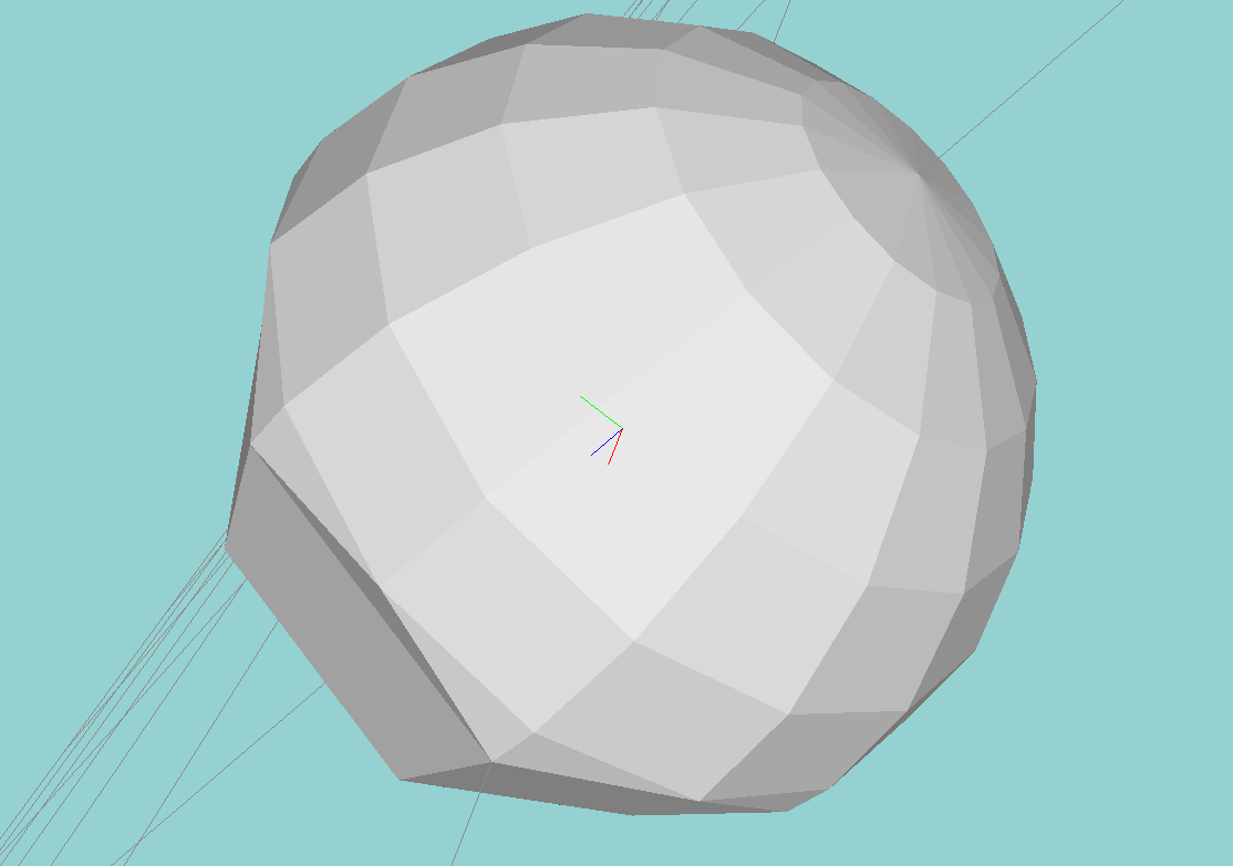
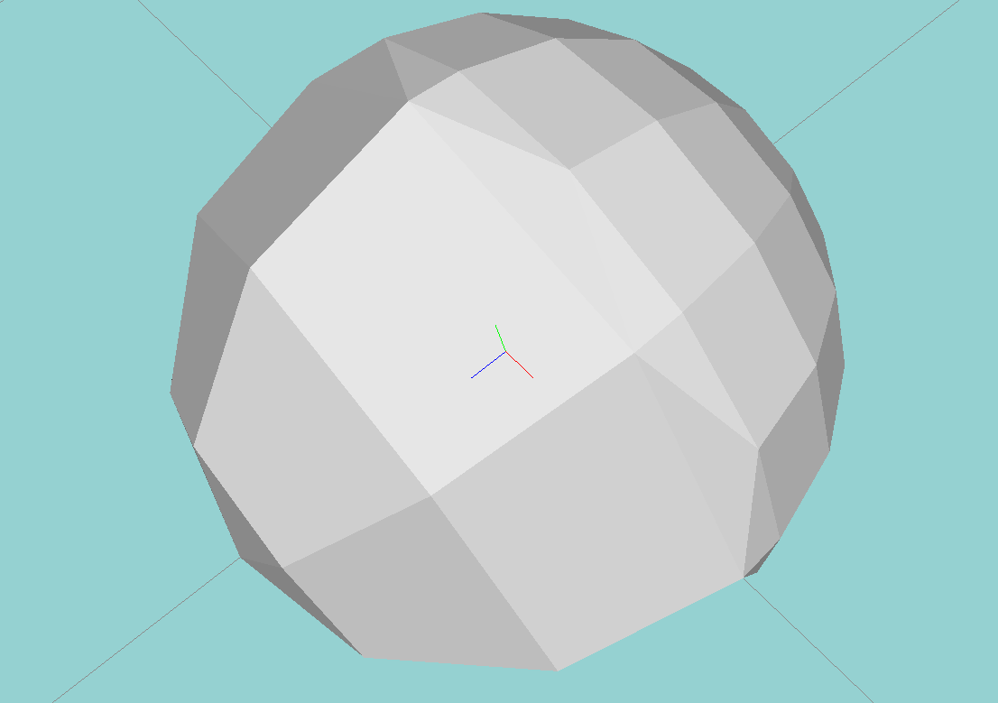
Two views of the “combination” resolution sphere, above. The finer-resolution part of the
sphere is where
,
while the coarser part of the sphere is where
.
You’ll then remove the factor of to make a new smoothing operator, which will end up being a “pure gradient” version of the “umbrella” operator.
This would no longer be an area or parameterization independent smoothing operator. You’ll apply this smoothing operator to the three spherical datasets, where we expect the uniform spheres to stay spherical, but the half-and-half “combination” sphere to become somewhat lopsided and distorted.
The interactive controls for your new smoothing program should be similar to your original smoothing program. Internally, it will be the same, other than the loss of the factor of from the calcuation.
To more clearly see the asymmetry, however, it may be necessary to render the images in wireframe, and also remove the rear-facing triangles from the rendering, where you don’t render the backfacing triangles.
Tell us how to run this program in your README file, and make screenshots to show the output with the original 1999 parameterization-independent smoothing operator and also with the new “pure gradient” version of the smoothing operator. You may need to rotate the view to make the screenshots more understandable.
We’re interested to see how large the effect can be, between the two types of smoothing, especially for the half-and-half “combination” sphere.
For other types of extra credit, explore more into the fields of geometry processing and discrete differential geometry, and implement a concept that you’re interested in. Some ideas include:
Of course, you can always pursue your own idea as well. Please consult with the TA’s ahead of time to make sure your extra credit topic is appropriate. Please also include details regarding your extra credit in the README. Extra credit points will be awarded based on the complexity of the work.
TA’s are not liable to help with extra credit.
What to Submit
Before submitting, please comment your code clearly and appropriately, making sure to give details regarding any non-trivial parts of your program (such as the building of the operator ).
Submit a .zip or .tar.gz file containing all the files that we would need to compile, run, and test your program. In addition, please submit in the .zip or .tar.gz a README with instructions on how to compile and execute your program as well as any comments and information that you would like us to know. The README is especially important if your program has significant issues, since we want to know what you have tried to debug; this will help us figure out how close you were at getting the program to work and give you a grade faster.
We ask that you name your .zip or .tar.gz file lastname_firstname_hw5.zip or lastname_firstname_hw5.tar.gz respectively, where you replace the “firstname” and “lastname” fields with your actual first and last name.
Please submit your zip or tar.gz to moodle in the area for Assignment 5.
Written by Kevin (Kevli) Li (Class of 2016).
Links: Home