The following will act as lecture notes to help you review the material from lecture for the
assignment. You can click on the links below to get directed to the appropriate section or
subsection.
Geometry processing, or alternatively known as mesh processing, is the study of theory and
algorithms for efficient analysis and manipulation of complex 3D models. The field heavily draws
concepts from applied mathematics and engineering in addition to computer science, and has a
wide range of applications that span from simple modeling for games and movies to modeling
for physical simulations, medical imaging, architectural design, and more. The field’s
ability to make accurate and precise looking visualizations of real-world phenomenon in
conjunction with computer graphics makes it a highly active and attractive area of current
research.
Closely related to geometry processing is the field of discrete differential geometry (DDG),
which looks at discrete analogs to notions in differential geometry – a branch of mathematics that
uses techniques from differential and integral calculus as well as linear algebra to study problems in
geometry. The field enables us to model and simulate in the discrete domain problems that would
normally involve smooth curves and surfaces. Hence, DDG focuses on finding discrete dualities to
continuous operations – such as differentiation and integration – that we can apply on
discrete constructs like line segments, polygons, and meshes. DDG goes hand-in-hand with
geometry processing in helping us computationally visualize complex sytems from our 3D
world.
These lecture notes aim to provide a cursory introduction to the fields of geometry processing and
DDG. We first present a ubiquitous data structure for representing geometry in these fields known
as the halfedge data structure. From there, we discuss the idea of solving Poisson equations
– which show up all over in mathematics and the physical sciences – in the discrete setting. During
this discussion, we touch upon the discrete Laplacian – one of the most important
discretizations in DDG – as well as the general process of building sparse matrixoperators. Building sparse matrix operators is an essential step in solving non-linearmatrix equations such as the Poisson equation. Finally, we end the notes with an
application of all the aforementioned concepts called implicit fairing, which smoothes the
surface of a given mesh. Because this is meant to be a cursory (i.e. high-level) overview,
we unfortunately omit a lot of the theoretical basis behind these concepts; the proofs
and analyses are outside the scope of an introductory computer graphics course and
are instead more appropriate for a discrete differential geometry course (see Caltech’s
CS177).
For those of you who are curious about the research in geometry processing and DDG or just want
to see some cool graphics, we refer you to the impressive works of Caltech’s own Peter Schröder
[1] and Keenan Crane [2], the latter of whom is now at Carnegie Mellon University. We also like to
thank Keenan Crane for his wonderful notes on “Digital Geometry Processing with Discrete
Exterior Calculus” [3], which motivated a lot of the content and provided the diagrams for these
notes.
The halfedge data structure is a space efficient representation of a triangle mesh that encodes
convenient incidence relationships among mesh elements – i.e. vertices, edges, and faces. In this
section, we introduce the halfedge data structure and discuss its utility and applications.
In particular, we go over how the halfedge is used to compute surface normals pervertex.
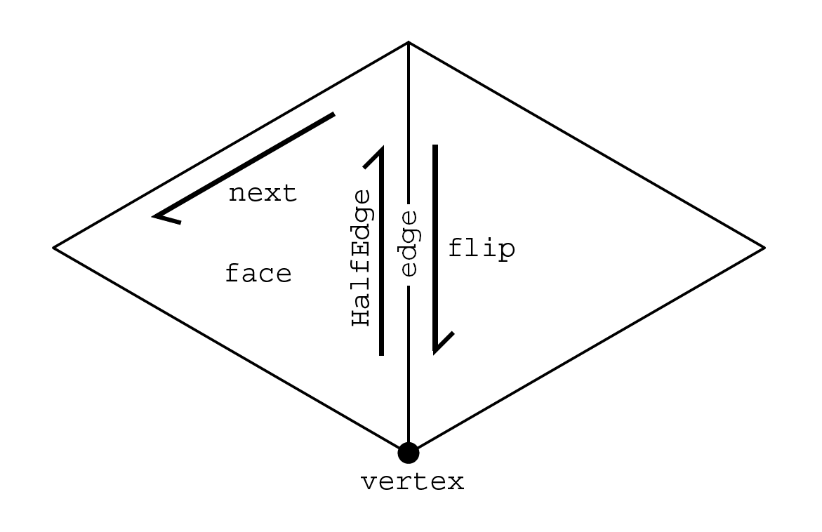
Consider Figure 1 and the following (pseudo)code snippet:
Figure 1: A visual of the halfedge data structure. Each halfedge contains a pointer to (1)
the vertex that it points away from, (2) the edge that it points along, (3) the face adjacent
to the halfedge, (4) the next halfedge, and (5) the flip halfedge on the other side of the
adjacent edge. The choices of which face we should associate with a halfedge and which
halfedge we should make the “next” are all based on how we orientate the halfedge when
we contruct it. These pointers provide a lot of flexibility for iterating over different mesh
regions. This diagram is taken from [3].
Conceptually, the halfedge is a directed edge in a triangle mesh. It is called the “halfedge” because
it constitutes only one direction of its adjacent edge; its flip halfedge makes up the other half. We
typically associate a halfedge with pointers to key mesh elements around it. The five key mesh
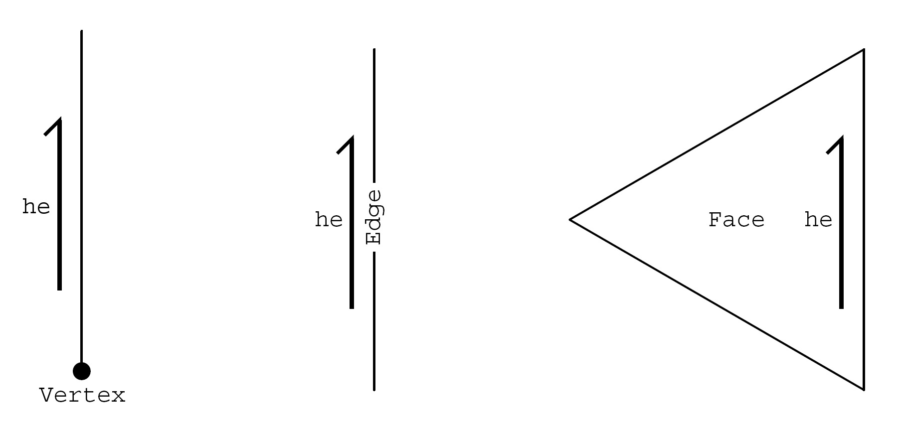
elements are shown in Figure 1. Each of these mesh elements stores a pointer to one of its
associated halfedges (Figure 2).
Figure 2: Each mesh element should contain a pointer to one of its associated halfedges.
This allows us to quickly access one mesh element given another mesh element via the
halfedge connections. For instance, we can access a nearby face given a vertex by going
vertex
halfedge
face. This diagram is taken from [3].
The network of pointers created by the halfedge and its associated mesh elements enables us to
conveniently iterate over different mesh regions. For instance, we can iterate over all the vertices
adjacent to a given vertex v in our mesh with a simple do-while loop:
Halfedge*he= v->halfedge; do { // do something with he->flip->vertex he= he->flip->next; } while( he!= v->halfedge )
Figure 3 shows a visual of the above loop running by numbering the vertices adjacent to
(our v) in the order that they would be traversed, starting with the halfedge from
to
vertex 1.
Figure 3: A visual of iterating over all vertices adjacent to
starting with the halfedge from
to vertex 1. The vertices adjacent to
are numbered in the order that they would be visited by our loop. This diagram is taken
and modified from [3].
As shown above, let v be , and
let the halfedge pointing from
to vertex 1 be the associated halfedge he. On our first iteration of the do-while loop, we
access he->flip->vertex, which we can see in Figure 3 to be vertex 1 (realize that
the flip of he would be pointing away from vertex 1 and so would be associated with
that vertex). Setting he to he->flip->next gives us the halfedge pointing from
to
vertex 2 for the next iteration. Eventually, as the loop goes on, he will be set back to the initial
halfedge, which is v->halfedge, and this completes our loop.
To drive home the power of the halfedge data structure, consider the work that we would have to
do to find all vertices adjacent to a given vertex v given a naïve mesh implementation – i.e. a
simple list of vertices and faces. We would first have to iterate over all faces to find
which ones v belong to; and from there, we would iterate over all the other vertices that
these selected faces contain. This process is by far less efficient than the simple do-while
loop we have above. Furthermore, it is quite difficult to discern any order among the
adjacent vertices with the naïve process, whereas the halfedge loop guarantees ordered
traversals.
As a final note, realize that the halfedge is very space efficient; it requires only the minimum
number of pointers to traverse an entire mesh. An alternative representation of a mesh that might
have been tempting is to simply have each vertex structure contain a list of pointers to all the
vertices that are adjacent to it. While this would functionally accomplish the same purposes as the
halfedge, it is much less space efficient, especially for larger meshes where we have many
connections among vertices.
For the purposes of this class, we have provided a simple, though a bit crude implementation of the
halfedge data structure found here. The comments in the header file detail how to use it. Note
that there are also many implementations of the halfedge on the internet; in particular,
Keenan Crane’s DDG library [3] has an excellent implementation, though it also has a lot
of dependencies – such as the matrix library Suitesparse – that are not trivial to set
up.
We are not actually going to cover how to implement the halfedge data structure in these notes. As
we might be able to imagine, the implementation process is quite complicated since we need to link
the halfedges to mesh elements appropriately so that we can traverse across the entire mesh by just
following halfedges. Ultimately, this class only requires you to know how to use the halfedge data
structure; knowing how to implement it among other details is useful, but not necessary for this
course. In practice, because there are various open source halfedge libraries nowadays, we rarely
need to make our own implementation.
Note that orientation of a surface is an important factor when using the halfedge. Since
halfedges traverse a mesh as a series of directed edges, the surface that the mesh represents
must be orientable – i.e. the surface has two sides that we can associate with positive
and negative directions. Essentially, we should be able to traverse the entire mesh by
following the halfedges without running into any conflicts (e.g. a halfedge’s flip points the
wrong way). Furthermore, the halfedge can only represent meshes where every edge is
contained in at most two faces; a more formal way to say this is that every edge must be
manifold.
Finally, meshes with boundaries – i.e. sets of edges that each only have one adjacent face –
require care when we handle them with the halfedge. For instance, we need to be careful when we
iterate over a mesh region that has a boundary, since we might try to process a face or vertex that
doesn’t exist. We defer the topic of boundaries to an actual DDG course. For this course, all themeshes that we work with have no boundary, so we do not have to worry aboutthis.
Back in Assignment 2, we said that we would defer the topic of computing surface normals to a
later assignment (i.e. this one). There are actually various methods for computing normals, each
with its own advantages and disadvantages. We are only going to cover one of these methods:
the area-weighted normal approach. It is one of the more commonly used methods
because of its simplicity and fast computation speed, but it does not always produce
the most accurate normals. Those who are curious about other, more sophisticated
methods for normal computation should refer to Chapter 5 of [3] or an actual DDG
course.
First, as a note of terminology, it is more appropriate to refer to our normals now as vertexnormals instead of surface normals, since we have a normal per vertex.
The area-weighted normal is a simple concept: for a given vertex, we compute the normal for
that vertex by taking a weighted vector sum of the normals of the incident faces; the weight
for each normal is the area of the associated face. This weighting scheme weights the
normals of smaller faces less and those of larger faces more. The area-weighted normal
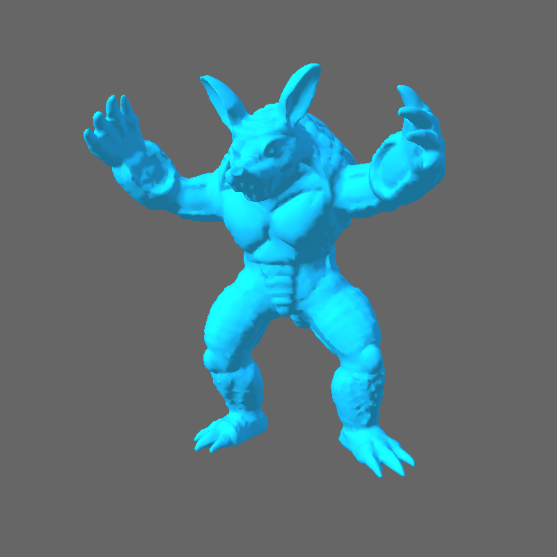
approach produces decent looking results in practice, such as those shown in Figure
4:
Figure 4: A Gouraud-shaded Stanford armadillo using area-weighted vertex normals.
To implement the computation for the area-weighted normal of a vertex v, we can simply build
upon the loop from subsection 2.1:
// initialize some vector structure, n, to the zero vector Halfedge*he= v->halfedge; do { Face*f= he->face; Vertex*v1= f->he->vertex; Vertex*v2= f->he->next->vertex; Vertex*v3= f->he->next->next->vertex; // face_normal = cross product of (v2 - v1) x (v3 - v1) // face_area = 1/2 | face_normal | // n += face_normal * face_area he= he->flip->next; } while( he!= v->halfedge ) // normalize n and return it
To get a better perspective on how this is applied in practice, let us consider how the loop iterates
over a non-planar triangle arrangement, as shown in Figure 5:
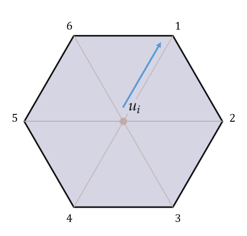
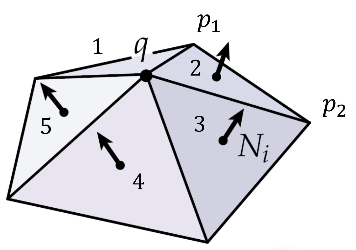
Figure 5: A visual of iterating over all faces incident to
starting with the halfedge from
to vertex
.
The faces incident to
are numbered in the order that they would be visited by our loop. For each iteration, we
compute the face area and face normal, using these values to compute the area-weighted
normal. This diagram is taken and modified from [3].
Let v be the vertex
in Figure 5 and the halfedge he be the directed edge from
to
. The
initial halfedge is adjacent to the face numbered 1, hence we process that face on the first
iteration of our loop. The step of he->flip->next takes us to the halfedge from
to
for
the next iteration; this halfedge is adjacent to the face numbered 2. The process goes
on, and just like before, our loop eventually brings us back to the initial halfedge and
terminates.
In this section, we discuss how to solve in the discrete domain the Poisson equation, which we
might remember from introductory physics as:
Recall from vector calculus and sophomore physics that
is the
Laplace operator, which gives us the divergence of the gradient of a scalar function. In physics,
might represent a given mass density, and solving the Poisson equation for
would yield a
gravitational potential. Or
might represent a given charge density, and solving for
would
yield an electric potential. It’s quite clear that the Poisson equation has key applications in
physics. But what may be surprising to know is that a number of problems in geometry processing
also involve solving a Poisson equation. One such problem is the smoothing of a surface via
implicit fairing, which we touch upon in the next section; for now, we discuss how we
represent and solve the Poisson equation in the discrete setting for our computer graphics
simulations.
To solve the Poisson equation in the discrete domain, we need to first develop a discreteLaplacian that approximates the effects of the continuous Laplace operator. That is, we want to
find a discrete method (or operation) such that – when it is applied to a function over the surface
of a mesh – it approximates the effects of the Laplacian being applied over a manifold (or a region
that is locally flat).
Similar to how there are various ways to compute vertex normals, there are actually various ways
to discretize the Laplacian; and all these methods have their own mathematical justification. In
their paper [4], Wardetzky et al. discuss how all these various discretizations of the Laplace
operator have their strengths and weaknesses depending on the application. We are going to go
over one of these approaches for the purpose of smoothing meshes via a technique known as
implicit fairing, which we discuss in the next section.
Recall that the Laplacian is defined to be the divergence of the gradient of a scalar function
:
That is, given a scalar function
and a point in space ,
evaluated
at gives us
evaluated at
. Looking at this
definition, we can think of the Laplacian as a generalization of the second derivative for functions defined over
. Now, we might
remember from vector calculus that we can parameterize any regular curve by arclength, which we denote
. Furthermore, recall
that the curvature
is given by:
where is a unit tangent
vector along the curve – i.e.
is a first derivative of our curve. Hence, curvature can be thought of as the magnitude of the
second derivative with respect to arclength. This establishes a connection between the Laplacian
and curvature.
Following this path of reasoning (though through a more rigorous means),
Desbrun et al. choose to approximate the Laplacian operator with the curvaturenormal operator [7]. Backing up a bit, the curvature normal – denoted
– for a
point
is given by the following defintiion from differential geometry:
(1)
where is the area of a small region
around where the curvature
is needed, and the gradient is
a gradient with respect to the
coordinates of . Let
be our discrete vertex
representation of the point .
Desbrun et al. discretized
by selecting the smallest possible area around the given vertex
, which
is the total area sum of the incident triangular faces.
Discretizing the gradient, ,
is a much more complicated procedure. Desbrun et al. provides an algebraic derivation of
in [7].
Keenan Crane provides a geometric derivation in Chapter 6 of [3]. Due to the length and
nontrivial prerequisites of both derivations, we omit the full, rigorous discretizations of
from
these notes (though we recommend those who are curious to read Keenan’s derivation of the
discrete Laplacian, as it mostly requires good geometric intuition). Both Desbrun et al. and
Keenan provide us the full discretization of Equation 1 as:
(2)
up to a scaling factor. Recall that
is the vertex at which we want to compute the curvature normal and
is the total area sum of the
incident faces to . The variable
is an index that iterates
over all vertices adjacent to .
The angles and
are the two angles opposite
to the edge formed by
and .
Figure 6 shows a visual of our angles:
Figure 6: A diagram depicting angles
and
for vertex
in Equation 2.
Equation 2 is famously referred to as the cotan formula and shows up everywhere in geometry
processing and DDG. The cotan formula computes the discrete curvature normal at a givenvertex of a mesh. Desbrun et al. and Keenan Crane show that the above cotanformula is a good approximation for the Laplacian of the individualposition functionsof a vertex .
Keenan Crane also does a more general derivation in Chapter 6 of [3] that gives us the
variant:
(3)
where denotes the
value of at a vertex
in the mesh, and
denotes the value
of the Laplacian of
evaluated at vertex .
Note the absence of the factorfor this cotan formula! The
factor is needed to compute the curvature and the normal vector, seen in the other equations,
which makes the curvature formula area independent.
Equation 3 is the general cotan formula for approximating the Laplacian of any scalarfunction ata vertex .
Now that we have a discretization of the Laplacian, how do we actually solve the Poisson equation in
the discrete domain? In other words, we are given a set of values, which are gotten from evaluating the
function
at various vertices on our discrete surface or mesh; and for each of these
values, we want to know
the corresponding
value based on the equation:
for each vertex .
From the previous subsection, we have a definition for the Laplacian in the discrete
domain:
which, when substituted into the Poisson equation, would give us:
The simplest way to solve this problem is to build matrix representations for
,
, and
and
set this up as a non-linear matrix equation. This enables us to then use a standardnumerical linear algebra library (like Eigen) to computationally solve for
.
To illustrate how this may work, let us consider solving a similar, but simpler
non-linear equation. Let us define the “distance-weighted-sum” operator
, which when
acting upon at
a given a vertex ,
computes the following weighted sum based on all neighboring vertices
:
For each vertex , the
operation gives us a sum
of the values of all vertices
adjacent to ; and for
each adjacent vertex , we
weight its value in the sum
by the edge length from
to .
Note that this distance-weighted-sum operator is very similar in form to the approximation of the
Laplacian given in Equation 3.
Now, let us define the following equation:
(4)
We are given a set of
values for each vertex
in our mesh, and we want to solve for all the corresponding
values, knowing
that the operator
is what maps the
values to
values. This is very similar to our standard Poisson problem, so if we know how to solve Equation
4, then we should be able to figure out how solve a Poisson equation.
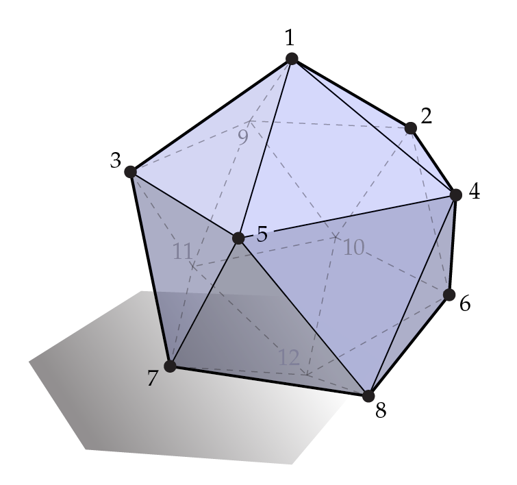
Let the mesh in Figure 7 be the surface upon which we are solving Equation 4:
Figure 7: The mesh for our example problem of solving Equation 4. This diagram is taken
from [3].
Given our mesh, we first need to index our vertices so that we know which vertex we meanwhen we say or .
Figure 7 already indexes the vertices of the mesh from 1 to 12.
Now, let us set up Equation 4 for just the first vertex,
. Since we need to find all
the vertices adjacent to ,
we can imagine how the halfedge data structure would be extremely useful here. Using
the techniques from Section 1, we can quickly iterate over each vertex adjacent to
; and for each adjacent vertex
, we can compute the edge
length and also retrieve
its value from our given
set of values. We can then
represent Equation 4 for
in the following matrix form:
Let us take a moment to convince ourselves that the above matrix equation correctly sets up Equation 4 for
. Looking at Figure
7, we see that vertex 1 is adjacent to vertices 2, 3, 4, 5, and 9. In the above equation, notice how we have a
value at every
th place of our 1x12
matrix whenever is
adjacent to in our
mesh. In all the th
places where is
not adjacent to
in our mesh, we put a 0. Expanding out the matrix multiplication on the left-hand side of our
equation, we should see that we have:
which is the correct Equation 4 for vertex .
We can similarly build matrix equations for ,
, ... ,
and
combine them all together into the following matrix equation:
(5)
Remember that we have the values of already, and we want to solve for the values of
. To do
this, we fall back on our friendly matrix library Eigen. Consider the following code
snippet:
#include<Eigen/Dense> #include<Eigen/Sparse> // function to assign each vertex in our mesh to an index voidindex_vertices( std::vector<Vertex*>*vertices ) { for(int i=1; i< vertices->size();++i )// start at 1 because obj files are 1-indexed vertices->at(i)->index= i;// assign each vertex an index } // function to construct our B operator in matrix form Eigen::SparseMatrix<double> build_B_operator( std::vector<Vertex*>*vertices ) { index_vertices( vertices );// assign each vertex an index // recall that due to 1-indexing of obj files, index 0 of our list doesnt actually contain a vertex int num_vertices= vertices->size()-1; // initialize a sparse matrix to represent our B operator Eigen::SparseMatrix<double> B( num_vertices, num_vertices ); // reserve room for 7 non-zeros per row of B B.reserve( Eigen::VectorXi::Constant( num_vertices,7 ) ); for(int i=1; i< vertices->size();++i ) { Halfedge*he= vertices->at(i)->halfedge; do// iterate over all vertices adjacent to v_i { int j= he->next->vertex->index;// get index of adjacent vertex to v_i // call function to compute edge length double edge_length= norm( he->vertex, he->next->vertex ); // fill the j-th slot of row i of our B matrix with appropriate value B.insert( i-1, j-1 )= edge_length; he= he->flip->next; } while( he!= vertices->at(i)->halfedge ); } B.makeCompressed();// optional; tells Eigen to more efficiently store our sparse matrix return B; } // function to solve Equation 4 void solve( std::vector<Vertex*>*vertices ) { // get our matrix representation of B Eigen::SparseMatrix<double> B= build_B_operator( vertices ); // initialize Eigens sparse solver Eigen::SparseLU<Eigen::SparseMatrix<double>, Eigen::COLAMDOrdering<int>> solver; // the following two lines essentially tailor our solver to our operator B solver.analyzePattern( B ); solver.factorize( B ); int num_vertices= vertices->size()-1; // initialize our vector representation of rho Eigen::VectorXd rho_vector( num_vertices ); for(int i=1; i< vertices->size();++i ) rho_vector(i-1)= rho( i );// assuming we can retrieve our given rho values from somewhere // have Eigen solve for our phi_vector Eigen::VectorXd phi_vector( num_vertices ); phi_vector= solver.solve( rho_vector ); // do something with phi_vector }
The first thing we should notice is that we are using a sparse matrix to represent our operator B.
This is because B is mostly filled with 0’s, as we can see from Equation 5. It would be a waste of space
– especially for larger meshes like the Stanford bunny – if we were to actually store all the elements
of in
memory when we know that most of them are 0. In fact, for much larger meshes like the Stanford
armadillo, we might actually run out of memory trying to store the entire operator. Hence, we
want to use a sparse matrix, which is a compact data structure for representing matrices that are
mostly filled with 0’s.
tells Eigen to reserve room in each row of B for at least 7 non-zero elements. This merely serves as
an initial estimate for the number of non-zero entries we expect per row. If we ever go over 7, Eigen
will reserve more space. Of course, reserving more space comes with some computational cost, so
it’s always best to over-estimate the number of non-zero entries we need per row. In practice, we’ve
found 7 to be a good starting number.
In the build_B_operator function, we see that we use the halfedge data structure
to help us find adjacent vertices and compute incident edge lengths for each vertex
. For each vertex
adjacent to
– denoted –
we fill the
slot of our
matrix with the appropriate edge length value. Of course, because Eigen matrices are 0-indexed, we need
to fill the
slot. Also notice how we need to index the vertices beforehand so that we associate each vertex with an
appropriate th
slot.
In the solve function, we construct vectors to represent
and
and a solver
based on our
matrix. Solving for
is then just a few simple lines of Eigen syntax. More details on the Eigen syntax can be found on
the official Eigen documentation for those who are curious.
Now that we know how to solve for
in Equation 4 using Eigen, can we extend our code to solve a Poisson equation? We leave this as an
exercise to the reader. The main difference is that we need to construct the discrete Laplacian instead
of our
operator; the rest of the logic is the same.
Finally, we end these notes with a discussion of one of the earliest applications of the discrete
Laplacian from Desbrun et al. [7]. In their paper, Desbrun et al. present a method known as
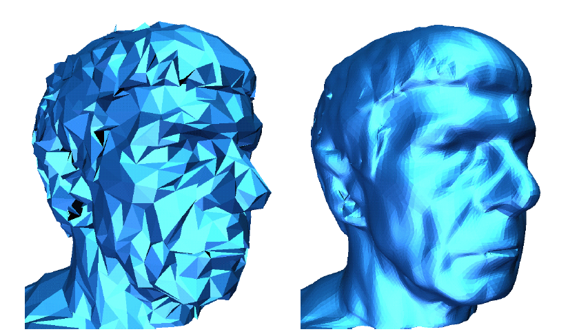
implicit fairing for smoothing the surface of a mesh. Figure 8 shows one result of this method
from the paper:
Figure 8: Implicit fairing of the coarse mesh on the left yields the smoothed mesh on the
right. This diagram is taken from [7].
The smoothing technique actually originates from a concept borrowed from physics and
engineering known as the heat equation, which describes how heat diffuses over a domain. The
heat equation is given by:
where
is a scalar function that describes the temperature at a point in space, and
represents time. Consider what this equation describes if
were in one
dimension (i.e. if
were a function of points on the real line). In one dimension, the Laplacian simplifies into
the second derivative, and the heat equation ends up saying that the rate of change of
is equal to its second derivative. So what would happen at points where
is
concave or convex? Recall from introductory calculus that when a function is concave, its second
derivative is negative. In the context of the heat equation, this means that concave bumps in
will fall flat over time
since the rate of change of
there is negative. Similarly, convex regions have positive second derivatives, so convex bumps rise
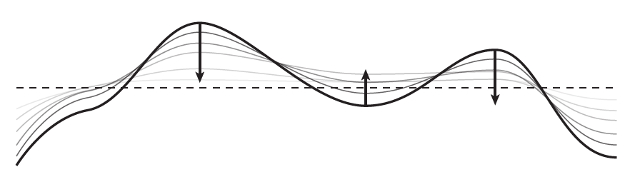
over time. Figure 9 shows a visual of this:
Figure 9: The heat equation for a 1D temperature function – such as the one shown –
says that concave bumps get pushed down over time while convex bumps get pushed up.
This diagram is taken from [3].
Hence, bumpy areas of
get smoothed out to be flat over time when governed by the heat equation.
Now consider what might happen if we replace the temperature function
with
vertex coordinates from a surface mesh. That is, we construct the following parallels to the heat
equation:
We would expect that these equations end up “smoothing” the
coordinates of the vertices, consequently getting rid of bumpy areas and smoothing the surface of
the mesh as a whole. In fact, this is exactly what happens; these equations are what we use toproduce the smoothing effect shown in Figure 8.
Using the equation for
as an example, let us show how we utilize the heat equation form to smooth a mesh. We start by
writing
as a finite difference:
where is some time
step, is the new
position after the
time step, and
is the original x position. We can then approximate our equation of interest as:
But what
do we use on our right-hand side? Suppose we were to use
for the
right-hand side. With some simple algebra, we obtain the following equation:
This gives us an explicit Euler – also known as forward Euler – equation that we can easily solve to
obtain the new
positions, , given
the original
positions, .
However, as we might remember from our introductory programming methods course, forward
Euler is numerically unstable, hence large time steps can cause solutions to have large error and
blow up.
An alternative option is to use
as the argument for the Laplacian – i.e. write:
With some algebra, we can express the above equation as:
(6)
where is the
identity matrix. Equation 6 is in the form of an implicit Euler, also known as backward Euler. For the
Laplacian ,
we can refer back to the variant expressed in Equation 3:
where we use the curvature normal to approximate the effects of Laplacian acting upon a vertex
position. Since we are dealing with smoothing of areas of high curvature, the curvature normal
approximation of the Laplacian is perfect for the task.
More rigorous details of why this variant that includes the factor of
of the
Laplacian is appropriate can be found in the paper by Desbrun et al. [7] or the notes by Keenan
Crane [3].
And there is a recent paper by Keenan Crane on another curvature smoothing method with some
improved properties, see [8], which uses a very different formulation.
Rewriting our Laplacian in the context of our problem yields the following equations involving the
Laplacian:
which are used respectively in the following equations:
Solving the above equations allows us to compute the new smoothed verticesgiven theold vertices .We can solve all three of these equations with the techniques that we discuss inSection 3 for solving the Poisson equation. Notice how the above three non-linear equations
are very similar to the Poisson equation; the operator is only slightly more complicated to build
than the standard Laplacian. Building the operator for these equations and using it to solve for
is left
as an exercise in the assignment.
The following movie shows the implicit fairing technique being used to smooth
the Stanford bunny. Each consecutive smoothing is the algorithm being run
again on the original mesh with twice the previous time step (starting at
):