Assignment 3 Lecture Notes

The following will act as lecture notes to help you review the material from lecture for the assignment. You can click on the links below to get directed to the appropriate section or subsection.

• Section 1: OpenGL
• Section 2: The Arcball
• Section 3: Quaternions
  • Quaternion Definitions
  • Rotations with Quaternions
• Section 4: The Arcball with Quaternions

Section 1: OpenGL

OpenGL (Open Graphics Library) is a cross-language, multi-platform API for rendering 2D and 3D graphics. It provides a plethora of functionality that automatically handles tedious graphics computations for us. For instance, all the matrix manipulations and the lighting and shading computations that you had to do manually in the previous two assignments are automatically done for us in OpenGL with some simple function calls.

For this class, we will be using OpenGL 3.0. It is not the newest version of OpenGL, but it is stable; and it contains all the necessary functionality for this class. Most of the syntax in OpenGL 3.0 carries over to the newer versions, so you should still be able to use more modern OpenGL without too much difficulty after this class. The main difference between OpenGL 3.0 and the newer versions is that OpenGL 3.0 depends on glut, which has been deprecated on Mac OS. Keep this in mind when looking into newer versions.

To help you learn how to write programs using OpenGL, we have provided a different kind of “lecture notes” than what you are used to. Rather than trying to explain OpenGL syntax on this webpage, we believe that it would be more effective to learn by seeing the syntax used in actual source code. Hence, the “lecture notes” for OpenGL are actually extensive, instructive comments in this demo program. This is the same demo program that we asked you to run previously to test your OpenGL environment, and it is also included within the Assignment 3 files.

As a note, the demo does not cover the OpenGL Shading Language (GLSL for short). GLSL will be covered in the next set of notes.

The comments and code are all in the opengl_demo.cpp file. You may consider the file to be a template for writing your own OpenGL programs.

Section 2: The Arcball

The Arcball is an intuitive method proposed by Ken Shoemake in 1992 for manipulating and rotating a scene with the mouse [1]. Ever since its introduction, the Arcball has become the primary mechanism that people use to rotate scenes and objects in a 3D computer environment. You may have already encountered the Arcball or variants of it if you have ever used popular modeling software such as Blender or many of Autodesk’s products. In this section, we discuss the details behind the Arcball mechanism and how to implement it with basic rotation matrices; the sections after this one discuss an alternative, more elegant way to implement the Arcball using a construct known as the quaternion.

The best way to get a sense of how the Arcball works is by seeing a demonstration, so let us begin by considering the following movie (if a picture is worth 1000 words, how many words is a movie worth?):

The above movie shows an OpenGL program that allows us to rotate a given scene with the mouse via the Arcball. In this case, the scene that we are rotating is a simple one that has the Stanford bunny mesh centered at the origin. You can see that, usually, when we click and drag the mouse from one point on the screen to another, the scene rotates in a direction that intuitively corresponds to the direction in which we move the mouse. And when we click and drag the mouse near the corners of the screen, the scene rotates only around an axis that perpendicularly intersects with the center of the screen. This gives us two different ways to rotate the scene with the mouse.

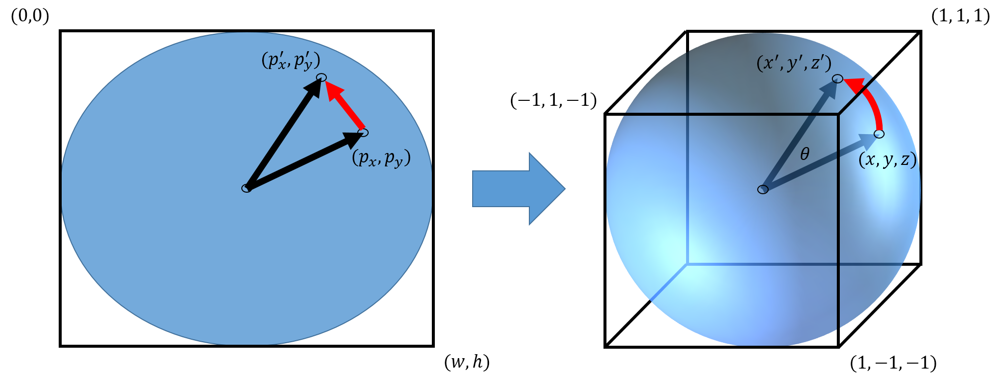
The Arcball works by trying to map a click-and-drag motion of the mouse on the screen to a rotation about the surface of a sphere of radius 1 that is inscribed into our viewing cube in NDC. Figure 1 shows a visual of this:

Suppose we click our mouse when it is at point $p=\left(p_x,p_y\right)$ on our screen in screen coordinates, and we move the mouse to another point $p^{\prime }=\left(p_x^{\prime },p_y^{\prime }\right)$ on our screen before we release the mouse button. The Arcball method first converts points $p$ and $p^{\prime }$ from screen coordinates to NDC, ignoring the missing z-component from the screen coordinates for now. Let us denote the NDC of $p$ and $p^{\prime }$ with $p_{ndc}=\left(x,y\right)$ and $p_{ndc}^{\prime }=\left(x^{\prime },y^{\prime }\right)$ respectively. From here, the Arcball computes z-coordinates for $p_{ndc}$ and $p_{ndc}^{\prime }$ by trying to map them to points on the surface of a sphere of radius 1, centerted at the origin of our NDC system. The z-coordinates of the two points are computed with the following function:

$$z=f\left(x,y\right)=\left\{\begin{array}{c}+\sqrt{1-x^2-y^2}\hfill \\ 0\hfill \end{array}\begin{array}{c},if\left(x^2+y^2\le 1\right)\hfill \\ ,if\left(x^2+y^2>1\right)\hfill \end{array}\right.$$

where the $+$ in front of the square root means that we take the positive root. Let us designate our two points now as $p_{ndc}=\left(x,y,z\right)$ and $p_{ndc}^{\prime }=\left(x^{\prime },y^{\prime },z^{\prime }\right)$, where $z$ and $z^{\prime }$ were computed using the above function.

The idea of the function is to map, if possible, the start and end points of our mouse motion on the screen to points on the surface of this inscribed sphere. Suppose both our start and end points ($p_{ndc}$ and $p_{ndc}^{\prime }$ respectively) are mapped onto the surface of the sphere successfully; i.e. $\left(x^2+y^2\le 1\right)$ and $\left({\left(x^{\prime }\right)}^2+{\left(y^{\prime }\right)}^2\le 1\right)$. The Arcball method then computes the rotation that transforms the position vector $p_{ndc}$ to the position vector $p_{ndc}^{\prime }$. Both these position vectors are shown in Figure 1.

As we have seen in computer graphics, a rotation can be defined in terms of an angle $\theta$ and a unit vector $u$ to rotate about. It is pretty straightforward to see that the rotation angle $\theta$ and rotation vector $v$ for our rotation of $p_{ndc}$ to $p_{ndc}^{\prime }$ are given by:

$$\theta =arccos\left(\frac{p_{ndc}\cdot p_{ndc}^{\prime }}{\left|p_{ndc}\right|\left|p_{ndc}^{\prime }\right|}\right)$$

$$u=p_{ndc}\times p_{ndc}^{\prime }$$

Remember to normalize $u$ to make it a unit vector. Also, be careful with floating and double point precision when computing arccos! Imperfect precision can cause the dot product within the arccos to slightly go above 1 (e.g. 1.00001), which would trigger a NAN from the arccos function. To safely compute arccos, we should take care to compute it as: arccos( min( 1 , arg ) ).

Once we have $\theta$ and $u$, we can form our usual axis-angle rotation matrix:

$$R=\left[\begin{array}{cccc}\hfill u_x^2+\left(1-u_x^2\right)cos\theta \hfill & \hfill u_x{u}_y\left(1-cos\theta \right)-u_{z}sin\theta \hfill & \hfill u_x{u}_z\left(1-cos\theta \right)+u_{y}sin\theta \hfill & \hfill 0\hfill \\ \hfill u_y{u}_x\left(1-cos\theta \right)+u_{z}sin\theta \hfill & \hfill u_y^2+\left(1-u_y^2\right)cos\theta \hfill & \hfill u_y{u}_z\left(1-cos\theta \right)-u_{x}sin\theta \hfill & \hfill 0\hfill \\ \hfill u_z{u}_x\left(1-cos\theta \right)-u_{y}sin\theta \hfill & \hfill u_z{u}_y\left(1-cos\theta \right)+u_{x}sin\theta \hfill & \hfill u_z^2+\left(1-u_z^2\right)cos\theta \hfill & \hfill 0\hfill \\ \hfill 0\hfill & \hfill 0\hfill & \hfill 0\hfill & \hfill 1\hfill \end{array}\right]$$

which we can use to rotate our scene.

One nice way to think about the Arcball is to imagine the scene that we see on our screen to be enclosed and set in-place within a sphere (or ellipsoid if the screen is not perfectly square). When we click and drag the mouse across the screen, we are essentially grabbing the sphere and rotating it about the center of the screen; and anything within the sphere rotates along with it.

In the event that the start and end points of our mouse motion fall outside the sphere in NDC, we still use the same process above for determining the rotation matrix. What will happen is that a z-component of 0 for the position vectors just simply results in a rotation about the z-axis (i.e. an axis coming out of the screen and through its center). This is what causes the two dimensional rotations that occur in the above movie when we click and drag near the corners of the gray screen.

In practice, when we implement the Arcball, we rotate the scene after every motion (i.e. change in screen coordinates) of the mouse that takes place between the initial click and the release of the mouse button. Using the method above, the OpenGL code structure for the Arcball would look something like the following:

where Compute_Rotation_Matrix() on line 15 is the procedure we describe above for computing the rotation matrix; and glMultMatrixd() on line 31 is the OpenGL function for transforming the current matrix mode (i.e. projection or modelview) by an arbitrary matrix, which is passed in as an argument. The passed-in matrix must be a pointer to a 4x4 column-major matrix structure. Luckily, the C++ matrix library, Eigen, already stores matrices in column-major, so we can simply pass in the data array of an Eigen matrix (e.g. my_matrix.data()) whenever we want to use glMultMatrixd().

The above code structure has the Arcball rotate scenes about the origin. This means though that scenes with translated cameras in the $x$ and $y$ directions will not rotate around the center of the screen, since the world origin wouldn’t correspond with the screen origin. This is often fine, because when we want to use the Arcball, it is usually to examine individual meshes; and in these situations, we would find it most convenient to center the mesh at the origin. Indeed, the Stanford bunny in the demo video above is centered at the origin to make it easier to examine with the Arcball.

As a final note for this section, we would like to point out that there is an alternative, more elegant way to implement the Arcball than the above-mentioned method. The alternative method is to compute and combine the rotations using a construct known as the quaternion instead of the usual axis-angle rotation matrices. One advantage that we can point out right now to using quaternions over rotation matrices is that it allows us to avoid the computational cost of constantly multiplying rotation matrices every render (line 31, which calls line 20, of Algorithm 1). We will see in the following sections that it is computationally more efficient to combine rotations using quaternions than rotation matrices.

Section 3: Quaternions

The quaternion is an extension of complex numbers that is often used in computer graphics for representing rotations. Its main uses in computer graphics are in interpolating rotations – which we will cover later in the class – and, of course, in the Arcball. The theory of quaternions is a large area of study, and we unfortunately cannot cover all of it within the scope of this class. Rather, we only present a cursory overview of the concept for the purposes of computer graphics. We do encourage those who are curious to look more into the matter on their own independent study.

Quaternion Definitions

A quaternion extends the idea of a complex number by adding two more “imaginary” components. While a complex number simply has a real and an imaginary ($i$) component, quaternions have a real component ($s$) and three “imaginary” components ($i,j,k$). We generally express quaternions in the following form:

$$q=s+xi+yj+zk$$

where $s,x,y,z\in ℝ$. People also often refer to the real component as the $w$-component instead of the $s$-component. Both $w$ and $s$ are commonly used, but for this class, we will use $s$.

The $i,j,k$ components of a quaternion satisfy the conditions:

$$i^2=j^2=k^2=ijk=-1$$

$$\begin{array}{c}ij=k\hfill \\ ji=-k\hfill \end{array}\begin{array}{c},jk=i\hfill \\ ,kj=-i\hfill \end{array}\begin{array}{c},ki=j\hfill \\ ,ik=-j\hfill \end{array}$$

We don’t need to worry about these conditions for the purposes of this class, but they are necessary for the definition of the quaternion. For those who are curious, the above relationships between the $i,j,k$ components correspond to the cross product relationships for the unit Cartesian vectors:

$$\begin{array}{c}x\times y=z\hfill \\ y\times x=-z\hfill \end{array}\begin{array}{c},y\times z=x\hfill \\ ,z\times y=-x\hfill \end{array}\begin{array}{c},z\times x=y\hfill \\ ,x\times z=-y\hfill \end{array}$$

We often find it convenient to represent quaternions as pairs of $\left[s,v\right]$, with $s\in ℝ,v\in {ℝ}^3$, and $v=xi+yi+zk$. Using this notation, we introduce the following basic arithmetic operations in the context of quaternions. Given two quaternions $q_a=\left[s_a,v_a\right]$ and $q_b=\left[s_b,v_b\right]$, we can perform quaternion addition and subtraction as follows:

$$q_a+q_b=\left[s_a+s_b,v_a+v_b\right]$$

$$q_a-q_b=\left[s_a-s_b,v_a-v_b\right]$$

Given a constant $c\in ℝ$, we also have scalar multiplication of a quaternion as follows:

$$c{q}_a=\left[c{s}_a,c{v}_a\right]$$

The product between two quaternions is given by:

$$q_a{q}_b=\left(s_a+x_{a}i+y_{a}j+z_{a}k\right)\left(s_b+x_{b}i+y_{b}j+z_{b}k\right)$$

$$=\left[s_a{s}_b-v_a\cdot v_b,s_a{v}_b+s_b{v}_a+v_a\times v_b\right]$$

where the first line can be simplified to the second line with some algebra.

Just like how a complex number has a complex conjugate, a quaternion $q$ has its own defined quaternion conjugate:

$$q^{*}=\left[s,-v\right]$$

As one might expect, the norm of a quaternion is given by:

$$\left|q\right|=\sqrt{s^2+x^2+y^2+z^2}$$

To normalize a quaternion into a unit quaternion, we simply divide the quaternion by its norm. Note that, similar to complex numbers, we also have the following relationship involving the conjugate and norm for quaternions:

$$q{q}^{*}=|q{|}^2$$

Finally, the inverse of a quaternion is defined as:

$$q^{-1}=\frac{q^{*}}{|q{|}^2}$$

If we multiply a quaternion by its own inverse, then we get the expected identity:

$$q{q}^{-1}=\left[1,0\right]=1$$

Rotations with Quaternions

In the context of rotations, quaternions give us a simple way to encode both the axis and angle of a rotation in a set of 4 numbers. Let $u=\left(u_x,u_y,u_z\right)=u_{x}i+u_{y}j+u_{z}k$ be the unit vector that represents our rotation axis of interest in ${ℝ}^3$, and let $\theta$ be the rotation angle. We define the corresponding quaternion for this rotation using an extension of Euler’s formula (i.e. $e^{i\theta }=cos\theta +isin\theta )$ as so:

$$r=e^{\frac{\theta }{2}\left(u_{x}i+u_{y}j+u_{z}k\right)}=cos\frac{\theta }{2}+\left(u_{x}i+u_{y}j+u_{z}k\right)sin\frac{\theta }{2}$$

$$=\left[cos\frac{\theta }{2},\left(u_{x}i+u_{y}j+u_{z}k\right)sin\frac{\theta }{2}\right]$$

To apply our rotation $r$ on a point $p=\left(p_x,p_y,p_z\right)\in {ℝ}^3$, we first represent $p$ as the quaternion $q=\left[0,p_{x}i+p_{y}j+p_{z}k\right]$, and then evaluate the conjugation of $q$ by $r$, defined to be:

$$q^{\prime }=rq{r}^{-1}$$

We can show through some algebra that $rq{r}^{-1}$ evaluates to $q^{\prime }=\left[0,p_x^{\prime }i+p_y^{\prime }j+p_z^{\prime }k\right]$, which contains the new, rotated position of our original point $p$ within the vector component of the quaternion. As a side note, it can also be shown that the conjugation operation can be algebraically simplified into the general axis-angle rotation matrix that we have been using throughout this class (i.e. one way to prove the correctness of our usual axis-angle rotation matrix is through quaternions).

To clarify the conversion between the axis-angle and quaternion representations of rotations, we explicitly list out the conversion equations below. Let our unit rotation axis be denoted with $u=\left(u_x,u_y,u_z\right)$, our rotation angle be $\theta$, and our unit quaternion be $q=\left[q_s,q_{x}i+q_{y}j+q_{z}k\right]$. Then:

$$\begin{array}{c}{q}_s=cos\frac{\theta }{2}\hfill \\ q_x=u_{x}sin\frac{\theta }{2}\hfill \end{array}\begin{array}{c},q_y=u_{y}sin\frac{\theta }{2}\hfill \\ ,q_z=u_{z}sin\frac{\theta }{2}\hfill \end{array}$$

And taking note that ${sin}^2\left(\frac{\theta }{2}\right)=1-{cos}^2\left(\frac{\theta }{2}\right)=1-q_s^2$, we have:

$$\begin{array}{c}\theta =2arccos\left(q_s\right)\hfill \\ u_x=q_x∕\sqrt{1-q_s^2}\hfill \end{array}\begin{array}{c},u_z=q_z∕\sqrt{1-q_s^2}\hfill \\ ,u_y=q_y∕\sqrt{1-q_s^2}\hfill \end{array}$$

The square root, arccos, and division in the last four equations are a bit discerning because they are functions known to lead to singularities. Thankfully, only the division can actually lead to a singularity.

Because $q$ is a unit quaternion, $q_s\le 1$, so we do not need to worry about the square root or inverse cosine returning anything but a real number. However, it is possible for the square root to be 0. If that were the case, then we would get a divide-by-zero when computing any of the axis components. This would be an issue if it were not for the fact that $0=2arccos\left(1\right)=\theta$. For the square root to be 0, $q_s$ must be 1. But if $q_s=1$, then $\theta =0$. This allows us to specify any arbitrary axis for $u$, since a rotation angle of $\theta =0$ means that we have no rotation at all. So in the event that the square root is zero, we can set $u$ to be any arbitrary axis.

It can also be shown that we can directly express a quaternion $q=\left[q_s,q_{x}i+q_{y}j+q_{z}k\right]$ as the following rotation matrix:

$$R=\left[\begin{array}{cccc}\hfill 1-2q_y^2-2q_z^2\hfill & \hfill 2\left(q_x{q}_y-q_z{q}_s\right)\hfill & \hfill 2\left(q_x{q}_z+q_y{q}_s\right)\hfill & \hfill 0\hfill \\ \hfill 2\left(q_x{q}_y+q_z{q}_s\right)\hfill & \hfill 1-2q_x^2-2q_z^2\hfill & \hfill 2\left(q_y{q}_z-q_x{q}_s\right)\hfill & \hfill 0\hfill \\ \hfill 2\left(q_x{q}_z-q_y{q}_s\right)\hfill & \hfill 2\left(q_y{q}_z+q_x{q}_s\right)\hfill & \hfill 1-2q_x^2-2q_y^2\hfill & \hfill 0\hfill \\ \hfill 0\hfill & \hfill 0\hfill & \hfill 0\hfill & \hfill 1\hfill \end{array}\right]$$

Finally, just like how we can combine rotations by multiplying their matrix representations together, we can also combine rotations by multiplying their quaternion representations together. That is, given two rotations represented by quaternions $q_1$ and $q_2$, the product:

$$q^{\prime }=q_2{q}_1$$

corresponds to the rotation obtained by first applying the rotation represented by $q_1$ and then applying the rotation represented by $q_2$. This is a much more elegant way of combining rotations than multiplying their axis-angle rotation matrices, which is more computationally expensive.

Section 4: The Arcball with Quaternions

Using what we know about quaternions, we can modify Algorithm 1 to produce a more efficient Arcball implementation:

This time, last_rotation and current_rotation are quaternions rather than rotation matrices. This makes line 20, which frequently gets called by line 31, less computationally expensive. Notice how the only matrix operation that occurs now is the mandatory OpenGL call to glMultMatrixd().

The structure of the code remains the same with only a couple of changes in the form of new functions. The Compute_Rotation_Quaternion() function computes the unit rotation axis and rotation angle based on the passed-in points and returns the quaternion that represents the rotation. The Get_Rotation_Matrix() function converts a given unit quaternion to a rotation matrix. For the latter function, it would be best to directly express the quaternion as the following rotation matrix:

$$R=\left[\begin{array}{cccc}\hfill 1-2q_y^2-2q_z^2\hfill & \hfill 2\left(q_x{q}_y-q_z{q}_s\right)\hfill & \hfill 2\left(q_x{q}_z+q_y{q}_s\right)\hfill & \hfill 0\hfill \\ \hfill 2\left(q_x{q}_y+q_z{q}_s\right)\hfill & \hfill 1-2q_x^2-2q_z^2\hfill & \hfill 2\left(q_y{q}_z-q_x{q}_s\right)\hfill & \hfill 0\hfill \\ \hfill 2\left(q_x{q}_z-q_y{q}_s\right)\hfill & \hfill 2\left(q_y{q}_z+q_x{q}_s\right)\hfill & \hfill 1-2q_x^2-2q_y^2\hfill & \hfill 0\hfill \\ \hfill 0\hfill & \hfill 0\hfill & \hfill 0\hfill & \hfill 1\hfill \end{array}\right]$$

This would be faster than converting the quaternion to its axis-angle representation and then forming the axis-angle rotation matrix; it also avoids the need to call the sine and cosine functions.

References

[1] http://dl.acm.org/citation.cfm?id=155312