Assignment 2 Lecture Notes

The following will act as lecture notes to help you review the material from lecture for the assignment. You can click on the links below to get directed to the appropriate section or subsection.

• Section 1: Triangle Interpolation
  • Barycentric Coordinates
  • Triangle Rasterization with Barycentric Coordinates
  • Triangle Interpolation with Barycentric Coordinates
  • Generalized Barycentric Coordinates
• Section 2: Lighting
  • Surface Normals
  • Diffuse Reflection
  • Ambient Reflection
  • Specular Reflection
  • The Lighting Model
  • Attenuation
• Section 3: Shading Algorithms
  • Gouraud Shading
  • Flat Shading
  • Phong Shading
• Section 4: Discarding Unnecessary Output
  • Depth Buffering
  • Backface Culling
• Section 5: Full Gouraud Shading Algorithm

Section 1: Triangle Interpolation

In computer graphics, we approximate the surfaces of solid objects by discretizing them as sheets of the simplest 2D surface: the triangle. We saw this to an extent in Assignment 1 where our wireframes consisted of many small triangle frames. We will now fill in these triangle frames to render solid surfaces.

To render a solid triangle, we find it convenient to assign information such as color to the triangle vertices and then interpolate this information across the triangle. For instance, to indicate that a right triangle face has a color gradient of say red to blue from the hypotenuse to the opposite point $p$, we would assign the color vector $\left[1,0,0\right]$ (i.e. 100% red, 0% green, 0% blue) to the endpoints of the hypotenuse and the color vector $\left[0,0,1\right]$ (i.e. 0% red, 0% green, 100% blue) to $p$. Interpolation then mixes the colors across the triangle to form the gradient.

There are a variety of interpolation schemes out there, but the simplest method is to use barycentric coordinates. We will develop these coordinates from scratch.

Barycentric Coordinates

Consider a triangle in 2D space with vertices $a,b,c$. From these vertices, we can form the vectors $\left(c-a\right)$ and $\left(b-a\right)$. Recall from basic linear algebra that we can span a 2D coordinate space given a point in the space and two linearly independent vectors. We know that the two vectors $\left(c-a\right)$ and $\left(b-a\right)$ have to be linearly independent; otherwise, the vertices $a$, $b$, and $c$ would not form a triangle. Hence, with point $a$ and basis vectors $\left(c-a\right)$ and $\left(b-a\right)$, we can express the coordinates of any point $p$ in the space as the following linear combination:

$$p=a+\beta \left(b-a\right)+\gamma \left(c-a\right)$$

for real coefficients $\beta$ and $\gamma$. We can then reorder the terms in the above equation to get:

$$p=\left(1-\beta -\gamma \right)a+\beta b+\gamma c$$

and define, for convenience, $\alpha =1-\beta -\gamma$ to rewrite the above equation as:

$$p=\alpha a+\beta b+\gamma c$$

with the constraint that:

$$\alpha +\beta +\gamma =1$$

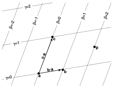
The barycentric coordinate system is the 2D space spanned by $\left(c-a\right)$ and $\left(b-a\right)$ with origin $a$. The vectors $\left(c-a\right)$ and $\left(b-a\right)$ are generally non-orthogonal. Figure 1 shows an example of a barycentric coordinate system:

We can compute the barycentric coordinates for an arbitrary point $p$ by rewriting:

$$p=a+\beta \left(b-a\right)+\gamma \left(c-a\right)$$

$$p-a=\beta \left(b-a\right)+\gamma \left(c-a\right)$$

as the following linear system:

$$\left[\begin{array}{cc}\hfill x_b-x_a\hfill & \hfill x_c-x_a\hfill \\ \hfill y_b-y_a\hfill & \hfill y_c-y_a\hfill \end{array}\right]\left[\begin{array}{c}\hfill \beta \hfill \\ \hfill \gamma \hfill \end{array}\right]=\left[\begin{array}{c}\hfill x_p-x_a\hfill \\ \hfill y_p-y_a\hfill \end{array}\right]$$

Solving for $\beta$ and $\gamma$ gives us:

$$\beta =\frac{\left(y_a-y_c\right)x_p+\left(x_c-x_a\right)y_p+x_a{y}_c-x_c{y}_a}{\left(y_a-y_c\right)x_b+\left(x_c-x_a\right)y_b+x_a{y}_c-x_c{y}_a}$$

$$\gamma =\frac{\left(y_a-y_b\right)x_p+\left(x_b-x_a\right)y_p+x_a{y}_b-x_b{y}_a}{\left(y_a-y_b\right)x_c+\left(x_b-x_a\right)y_c+x_a{y}_b-x_b{y}_a}$$

Once we have $\beta$ and $\gamma$, we can compute $\alpha$ using the definition:

$$\alpha =1-\beta -\gamma =\frac{\left(y_b-y_c\right)x_p+\left(x_c-x_b\right)y_p+x_b{y}_c-x_c{y}_b}{\left(y_b-y_c\right)x_a+\left(x_c-x_b\right)y_a+x_b{y}_c-x_c{y}_b}$$

Note that the equations for $\alpha$, $\beta$, and $\gamma$ all have similar numerators and denominators. We can use this fact to our advantage to simplify our implementation of barycentric coordinates. Consider the following function:

$$f_{ij}\left(x,y\right)=\left(y_i-y_j\right)x+\left(x_j-x_i\right)y+x_i{y}_j-x_j{y}_i$$

We can express the equations for $\alpha$, $\beta$, and $\gamma$ in terms of $f_{ij}$ in the following manner:

$$\alpha =\frac{f_{bc}\left(x_p,y_p\right)}{f_{bc}\left(x_a,y_a\right)}$$

$$\beta =\frac{f_{ac}\left(x_p,y_p\right)}{f_{ac}\left(x_b,y_b\right)}$$

$$\gamma =\frac{f_{ab}\left(x_p,y_p\right)}{f_{ab}\left(x_c,y_c\right)}$$

The above representations allow us to compute barycentric coordinates by simply implementing the function $f_{ij}$ and calling it repeatedly with the appropriate parameters.

Triangle Rasterization with Barycentric Coordinates

The power and convenience of barycentric coordinates will become evident once we analyze them for a point inside the original triangle that we used to establish the coordinates.

First, consider what happens to $\alpha$, $\beta$ and $\gamma$ for a point inside the triangle formed by vertices $a$, $b$, and $c$ back in Figure 1. It is obvious that $\beta$ and $\gamma$ must be between 0 and 1. The line segment $\overline{bc}$ can be expressed as part of the line $\gamma =-\beta +1$ or more usefully as $\beta +\gamma =1$ in barycentric coordinates. If $\overline{bc}$ is part of $\beta +\gamma =1$, then the area to the left of $\overline{bc}$, including the entire area of the triangle, must be $\beta +\gamma <1$. And if $\beta +\gamma <1$ is true for a point inside the triangle, then $\alpha =1-\beta -\gamma$ must be between 0 and 1. Hence, a point is only inside a triangle if and only if its barycentric coordinates for that triangle obey the following inequalities:

$$0<\alpha <1$$

$$0<\beta <1$$

$$0<\gamma <1$$

It is straightforward to also see that for a point directly on an edge of the triangle, the two barycentric coordinates associated with the edge endpoints must be between 0 and 1 while the remaining coordinate must be 0. And for a vertex of the triangle, the barycentric coordinate associated with that point must be 1 while the other two must be 0.

The above results can be used to devise an algorithm that determines which pixels in a pixel grid to fill when rasterizing a triangle. Given the triangle vertices in screen coordinates, we would first find the bounding box for the three vertices - i.e. we find the smallest rectangle of pixels in the grid that encompasses all three vertices. From there, we consider each pixel within the bounding box and compute its barycentric coordinates using the vertices of the triangle. We use the barycentric coordinates to determine whether the pixel is inside or on an edge of the triangle and fill in the pixel if either case is true.

Triangle Interpolation with Barycentric Coordinates

We next look at what barycentric coordinates are mainly used for in computer graphics: interpolating arbitrary values across a triangle. Consider how we linearly interpolate a value $v$ located at $x$ in some 1D space between two values $v_1$ located at $x_1$ and $v_2$ located at $x_2$:

$$v=\frac{x_2-x}{x_2-x_1}{v}_1+\frac{x-x_1}{x_2-x_1}{v}_2$$

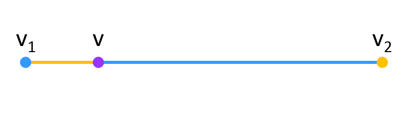
We assign a weight to one of the known values $v_i$ in our weighted sum based on the distance between the unknown value $v$ and the other known value $v_j$. As a result, the closer $v$ is to $v_i$, the larger the weight assigned to $v_i$ becomes. And the further away $v$ is to $v_i$, the smaller the weight becomes. Figure 2 shows a visual of this:

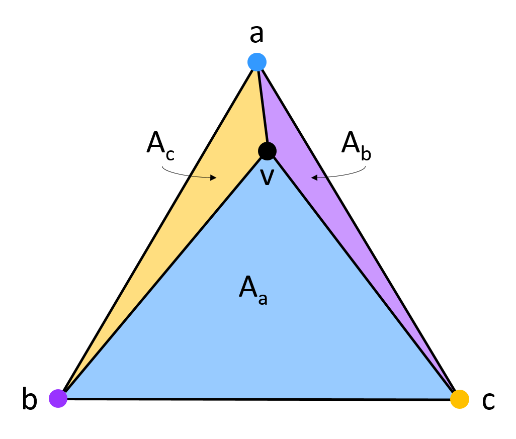
Interpolating a value $v$ among three values $a,b,c$ uses the same idea of assigning weights, except it bases the weights on areas instead of one-dimensional distances. Consider Figure 3:

Let $A$ be the area of triangle $abc$ in Figure 3. Then our weighted sum for interpolating $v$ is:

$$v=\frac{A_a}{A}a+\frac{A_b}{A}b+\frac{A_c}{A}c$$

It turns out that we can compute the areas $A_a,A_b,A_c,$ and $A$ using the barycentric coordinates for $v$. Let us assign each value an appropriate ordered pair $\left(x,y\right)$ in Cartesian coordinates. Recall from basic geometry that the area of a triangle with vertices $a,b,c$ is given by the following determinant:

$$A_{abc}=\frac{1}{2}\left|\begin{array}{cc}\hfill x_b-x_a\hfill & \hfill x_c-x_a\hfill \\ \hfill y_b-y_a\hfill & \hfill y_c-y_a\hfill \end{array}\right|=\frac{1}{2}\left(x_a{y}_b+x_b{y}_c+x_c{y}_a-x_a{y}_c-x_b{y}_a-x_c{y}_b\right)$$

Let us compute the area of triangle $avc$ in Figure 3:

$$A_{avc}=A_b=\frac{1}{2}\left|\begin{array}{cc}\hfill x_v-x_a\hfill & \hfill x_c-x_a\hfill \\ \hfill y_v-y_a\hfill & \hfill y_c-y_a\hfill \end{array}\right|=\frac{1}{2}\left(x_a{y}_v+x_v{y}_c+x_c{y}_a-x_a{y}_c-x_v{y}_a-x_c{y}_v\right)$$

The weight assigned to vertex $b$ in the interpolation is then:

$$\frac{A_b}{A}=\frac{x_a{y}_v+x_v{y}_c+x_c{y}_a-x_a{y}_c-x_v{y}_a-x_c{y}_v}{x_a{y}_b+x_b{y}_c+x_c{y}_a-x_a{y}_c-x_b{y}_a-x_c{y}_b}$$

The expression on the right-hand side should look familiar. Recall the formula we got for $\beta$ and fully expand the products:

$$\beta =\frac{\left(y_a-y_c\right)x_p+\left(x_c-x_a\right)y_p+x_a{y}_c-x_c{y}_a}{\left(y_a-y_c\right)x_b+\left(x_c-x_a\right)y_b+x_a{y}_c-x_c{y}_a}=\frac{x_a{y}_c+x_p{y}_a+x_c{y}_p-x_a{y}_p-x_p{y}_c-x_c{y}_a}{x_a{y}_c+x_b{y}_a+x_c{y}_b-x_a{y}_b-x_b{y}_c-x_c{y}_a}$$

Factor out a negative sign from both the numerator and denominator of the right-hand side expression in the above equation and replace $p$ with $v$ to get:

$$\beta =\frac{x_a{y}_v+x_v{y}_c+x_c{y}_a-x_a{y}_c-x_v{y}_a-x_c{y}_v}{x_a{y}_b+x_b{y}_c+x_c{y}_a-x_a{y}_c-x_b{y}_a-x_c{y}_b}=\frac{A_b}{A}$$

It can be shown through similar means that:

$$\gamma =\frac{A_c}{A}$$

$$\alpha =\frac{A_a}{A}$$

Hence, we can simply interpolate our unknown value $v$ as:

$$v=\alpha a+\beta b+\gamma c$$

just like how we would interpolate the coordinates of a point $p$ within a triangle. This should not be too surprising of a fact, since when we started to consider the values $a,b,c,v$ under a Cartesian coordinate system, we reduced the problem of interpolating $v$ to the problem of interpolating the coordinates of a point $p$ in a triangle.

The important lesson here is that barycentric coordinates allow us to interpolate any unknown value among three known values. We could, for instance, use them to interpolate the color of a point $p$ in triangle $abc$:

$$R_p=\alpha R_a+\beta R_b+\gamma R_c$$

$$G_p=\alpha G_a+\beta G_b+\gamma G_c$$

$$B_p=\alpha B_a+\beta B_b+\gamma B_c$$

where $R,G,B$ refer to the red, green, and blue color values. Let us now update the algorithm that we devised earlier to include color interpolation.

Do note that this algorithm does not properly handle pixels whose centers are exactly on an edge shared between two adjacent triangles. There is no obvious way to associate the pixel with one of the triangles over the other. The above algorithm does not bother to make any sophisticated decisions and instead draws any shared edges twice, with the edge of the second triangle overwriting the edge drawn for the first triangle. In practice, this is not that big of an issue, since adjacent triangles in our solid objects tend to not differ too drastically in color.

However, there are various heuristics out there that try to assign pixels on shared edges appropriately to only one of the two triangles. Unfortunately, these heuristics are outside the scope of the class. For those who are curious, pages 168-169 of [1] present an overview of one possible heuristic.

Generalized Barycentric Coordinates

While barycentric coordinates are mostly used with triangles, they have also been generalized for n-sided polygons. This generalization is outside the scope of this class, but for those who are interested, we have provided a link [2].

Section 2: Lighting

To achieve a 3D effect when we render surfaces, we use lighting and shading. In this section, we will talk about lighting; we cover shading in the next section.

The most commonly used lighting model is the Phong reflection model, also known simply as the lighting model. This model is often ambiguously referred to as Phong shading even though there is also the Phong shading algorithm, which we will cover in a later section. To avoid ambiguity, many people simply refer to the model as the lighting model. For this class, we will also refer to it as the lighting model, and like with barycentric coordinates, we will develop the model here from scratch.

Surface Normals

All lighting and shading calculations involve unit surface normals. So before we get into the lighting model, we need to first discuss unit surface normals in computer graphics.

Recall from multivariable calculus that the unit surface normal at a point $P$ on a surface is defined to be the unit vector pointing in the direction perpendicular to the tangent plane at $P$. This definition causes some issues for when we represent parts of curved surfaces as flat triangles in computer graphics. For a curved surface like a spherical shell, each point on the surface has its own different unit surface normal, since each point has its own different tangent plane. However, for a flat surface like a triangle, each point on the surface shares the same unit surface normal, since all the points share the same tangent plane. This difference poses the question of how we should represent unit surface normals on our discretized surfaces. Should we still treat our triangulated surfaces as though it were still the original curved surface, or do we treat each discrete triangle as an individual flat surface?

To render realistic lighting, we need to still treat triangulated surfaces as though it were still the original curved surface. This means that each of the three vertices of a triangle in our discretization of say a spherical surface has a different unit surface normal, even though the vertices are all part of the same flat triangle. This may seem unintuitive, but in this case, we need to treat our discretizations as though they were non-discretizations in order to portray realism.

We will cover how to compute the unit surface normals for points on a discretized surface in a later assignment. For now, we will assume that we are provided the unit surface normals whenever we need them for a computation.

As we might expect, the unit surface normals for points inside a triangle on our discretized, curved surfaces can be computed by interpolating the unit surface normals of the three triangle vertices using barycentric coordinates.

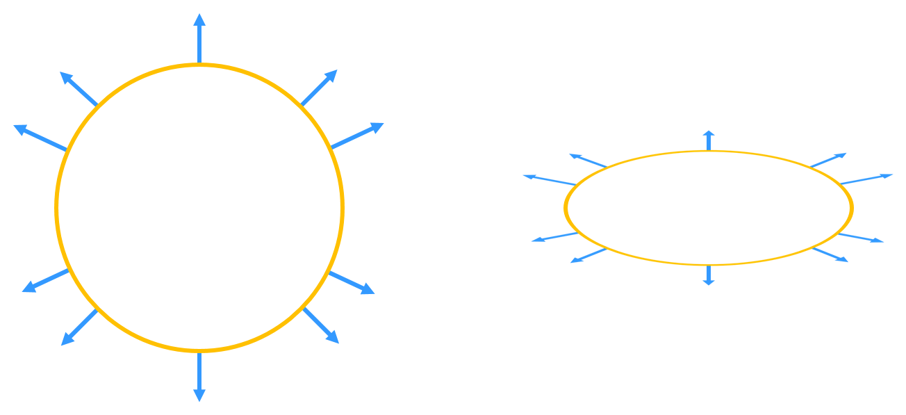
Transforming normals is a bit different from transforming points in world space. First, it is clear to see that translations are irrelevant for normals. We can translate a normal all we want, but the normal will still be the same vector. Rotations and scalings still have an effect, but we cannot simply apply them to normals the same way that we would to point coordinates. Consider, for instance, a non-uniform transform that scales each axis by a different factor in such a way as to “stretch” a circle into an ellipse as in Figure 4:

The vectors displayed on the ellipse are what we would expect if we transformed the original normals of the circle by the matrix we used to transform the circle itself. However, we can clearly see that not all the vectors on the ellipse are perpendicular to their incident tangent planes, and hence, they are not proper normals.

We have to derive a different transformation scheme that properly transforms the original normal $n$ for a point $p$ on a surface to the new normal $n^{\prime }$ for $p^{\prime }$ on the transformed surface. Note that because translations are irrelevant, we have no need for the fourth row or column in any normal transformation matrix. Hence, we only need to work with 3x3 matrices when dealing with normals.

Let $X$ be the normal transformation matrix that we are trying to find - i.e. $n^{\prime }=Xn$. Let $t$ be the tangent plane incident to $p$ and hence perpendicular to normal $n$. Let $M$ be the overall 3x3 transformation matrix (neglecting translations as they are irrelevant) such that $t^{\prime }=Mt$ is the transformed tangent plane. Since $n^{\prime }$ and $t^{\prime }$ are perpendicular, we can write:

$$n^{\prime }\cdot t^{\prime }=\left(Xn\right)\cdot \left(Mt\right)=0$$

Then, using properties of transposes and the associative property of matrix multiplication:

$$n^{\prime }\cdot t^{\prime }=\left(Xn\right)\cdot \left(Mt\right)=0$$

$$={\left(Xn\right)}^T\left(Mt\right)=0$$

$$=\left(n^T{X}^T\right)\left(Mt\right)=0$$

$$=n^T\left(X^{T}M\right)t=0$$

We can clearly see that the above equation is satisfied if $\left(X^{T}M\right)=I$, the identity matrix, since $n^{T}t=n\cdot t=0$. Solving for $X$ from $\left(X^{T}M\right)=I$ gives us:

$$X={\left(M^{-1}\right)}^T$$

Hence, to transform normals appropriately, we use the inverse transpose of the transformation matrix we use for points, neglecting the translation components.

For instance, suppose our transformations for our points in world space consist of a translation $T$, followed by a rotation $R$, followed by a scaling $S$. The matrix we would use to transform our normals then would be:

$$X={\left({\left(SR\right)}^{-1}\right)}^T$$

As a final note, any calculations involving surface normals should always be done in world space. This includes the computations in the lighting model and the shading algorithms in the following section. The math behind these calculations were all made in standard Cartesian coordinates and not the warped, camera and perspective coordinates.

Diffuse Reflection

The first component of the lighting model is diffuse reflection. Diffuse reflection is the reflection of light off a surface at many angles; the incident ray hits the surface and out forms many scattered, reflected rays at various angles. This causes the effect where the color and brightness of a point on a surface appears relatively constant despite changes in our viewpoint. Objects that primarily reflect diffuse light include paper, unfinished wood, and unpolished stones. We model diffuse reflection by considering the characteristics of an ideal diffuse reflecting surface, which reflects incoming light equally at all angles. An ideal diffuse reflecting surface is also known as a Lambertian surface, hence, the model we use for diffuse reflection is known as Lambertian reflectance.

A Lambertian surface obeys Lambert’s cosine law, which states that the luminous intensity of a point $p$ on the surface is proportional to the cosine of the angle $\theta$ between the incident light ray and surface normal. For our purposes, luminous intensity is equivalent to magnitudes of RGB color values. Hence, letting $c=\left[r,g,b\right]$ be our color vector of RGB values, we have:

$$c\propto cos\theta$$

Letting $l$ be the unit vector in the direction of the light from $p$ and $n$ be the unit surface normal at $p$, we can express the cosine as the following dot product:

$$c\propto n\cdot l$$

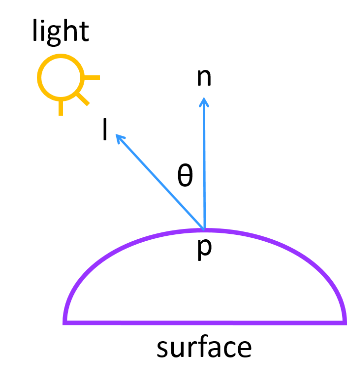
Figure 5 shows a diagram of the vectors involved in the calculation:

The color of our point should also depend on the surface’s diffuse reflectance, an inherent property of the material that determines the fraction of incoming diffuse light reflected by the surface. The fraction is different for each wavelength of light; or in our case, it is different for each color component. Let $c_d=\left[r_d,g_d,b_d\right]$ be our vector of fractional values for diffuse reflectance. Then:

$$c\propto c_{d}cos\theta$$

Finally, the magnitude of our color values should depend on the intensity of the light as well. Let $c_l$ be our vector of fractional values that determine the fraction of outgoing light (i.e. each color component of outgoing light) from the light source. Then:

$$c=c_d{c}_{l}n\cdot l$$

The above equation is our model for diffuse reflectance. However, we need to be cautious of the dot product, since it can be negative for cases where the surface normal $n$ points away from the light source. In these cases, the surface should recieve no light illumination (i.e. $c=\left[0,0,0\right]$) because it is not facing the light. We can account for these cases with a max function:

$$c=c_d{c}_{l}max\left(0,n\cdot l\right)$$

Ambient Reflection

We cannot solely use diffuse reflection as our lighting model because points whose normals point away from the light(s) will be colored entirely black. However, in reality, there will always be some light reflected off the surroundings to illuminate even the surfaces that face away from the light(s). We refer to this lighting as ambient light and its reflection as ambient reflection.

Let us consider how ambient light interacts with a single point on a sufrace. Since ambient light has been reflected and scattered so much by the environment, it appears to come from all directions as it hits the point. Hence, we model ambient light as though it is incoming from all directions. Additionally, very little ambient light often reaches our eyes after bouncing off the environment. As a result, points illuminated by just ambient light appear to have constant color even when we change our viewpoints, just like points illuminated by only diffuse light on a Lambertian surface. Thus, we also take ambient light to be reflected equally in all directions.

Since ambient light has absolutely no directional or single light source dependence, we can represent it in our lighting model by solely looking at how much ambient light a surface reflects. That is, given a particular surface, we just need to look at its ambient reflectance, an inherent propety of the material that determines the fraction of incoming ambient light reflected by the surface. The concept is very similar to diffuse reflectance. Let $c_a$ be our vector of fractional values for a surface’s ambient reflectance. We factor $c_a$ into the diffuse reflection model from the previous subsection:

$$c=c_a+c_d{c}_{l}max\left(0,n\cdot l\right)$$

Note that the sum may result in a color vector with components greater than 1. In these cases, we would need to clamp any components over 1 down to 1, as we cannot have over 100% of a color component.

Specular Reflection

The final component of the lighting model accounts for specular highlights, the bright spots of light that appear on illuminated shiny objects. If we were to look carefully at specular highlights in real life, we would see that they are simply direct reflections of light. Hence, to model specular reflection on a given surface for a given light source, we would need to create a bright spot on the surface such that the center of the spot is the point where the direction of the camera vector $e$ lines up with the direction of light reflection, which we will represent as vector $r$. This would model the direct reflection of light to our eyes produced by real specular highlights. We use $e$ here instead of $c$ for the camera vector due to $c$ already referring to color vectors, and $e$ is often used when people refer to the camera space by its equivalent eye space name.

To model the size of the bright spot, we would like some sort of function that causes the color at a point on our surface to be bright when $e=r$ and dim as $e$ moves away from $r$. The natural thing to do would be to have the function depend on the cosine of the angle between $e$ and $r$ - i.e. the color is brightest when the cosine is 1 and dimmest when the cosine is 0. Letting $e$ and $r$ be unit vectors, we can express the cosine as a dot product. Also, similar to diffuse reflection, specular reflection should factor in the color of the incoming light from the light source and the specular reflectance $c_s$ of the surface material. Putting all these factors into one formula gives us:

$$c_{specular}=c_s{c}_l\left(e\cdot r\right)$$

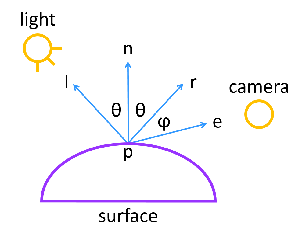
Figure 6 shows a diagram of the vectors involved in the calculation:

Like with the dot product in our diffuse reflection model, we need to account for negative values using a max function. Also, it turns out that, in practice, the above formulation actually results in a specular highlight that is much wider than what we would see in real life. The maximum color and brightness of the center point turn out correct, but the radius of the highlight is too big. To address this issue, we can dampen the brightness of the color much faster as the angle between $e$ and $r$ increases by raising the dot product to a positive, real number exponent:

$$c_{specular}=c_s{c}_{l}max{\left(0,e\cdot r\right)}^p$$

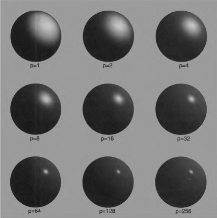
We call $p$ the Phong exponent $p$ is also referred to as the shininess value and is treated as a propety of the surface material. For instance, a very shiny surface like polished metal would have a $p$ value close to 1. Figure 7 shows the effect that $p$ has on the size of the specular highlight:

Computing the dot product in our model is not trivial though since we have to compute $r$. A cleaner way to accomplish what we want is to actually use the vector halfway between $e$ and $l$. Call this vector $h$. Then when $e$ lines up with $r$, $h$ should line up with the surface normal vector $n$. Hence, the cosine of the angle between $n$ and $h$ can be used instead of the cosine of the angle between $e$ and $l$. 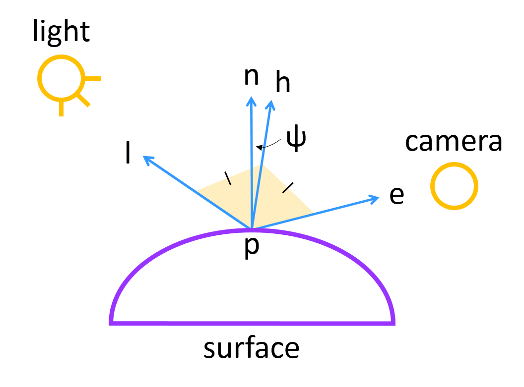Figure 8 shows a visual of the vectors:

The unit vector $h$ can be computed simply as:

$$h=\frac{e+l}{|e+l|}$$

And our specular reflection model becomes:

$$c_{specular}=c_s{c}_{l}max{\left(0,n\cdot h\right)}^p$$

$$=c_s{c}_{l}max{\left(0,n\cdot \frac{e+l}{|e+l|}\right)}^p$$

The Lighting Model

Finally, we add in the specular reflection to our diffuse and ambient reflection model to form the complete lighting model:

$$c=c_a+c_d{c}_{l}max\left(0,n\cdot l\right)+c_s{c}_{l}max{\left(0,n\cdot \frac{e+l}{|e+l|}\right)}^p$$

This leads us to an algorithm for computing the color of a point $P$ on an illuminated surface. The parameters for the algorithm are as follows:

• The position of the point $P$ as a triple of $\left(x,y,z\right)$ coordinates.
• The surface normal $n$ as a vector of $\left(x,y,z\right)$ components.
• The material reflectance and shininess properties, all of which are stored in the material parameter.
• The list of light sources, which we will call lights.
• The camera position $e$ as a triple of $\left(x,y,z\right)$ coordinates.

The algorithm itself is as follows:

Note that we use cwise_min and $\circ$ in line 23 to denote the component-wise min function and component-wise product of two vectors respectively.

Recall that all calculations involving normals should be done in world space. Hence, these lighting and color calculations should be done before any camera and perspective transformations. Also note how the above algorithm uses triples of $\left(x,y,z\right)$ rather than homogeneous coordinates. This does not matter too much since the homogeneous $w$ components of our coordinates in world space should all be 1, so we can just ignore the $w$ values. However, it is something to keep in mind when implementing the algorithm.

Attenuation

The lighting model does not take into account the distance between a light source and the point that is being processed. However, in real life, moving a light source further away from a point should dim the amount of light that illuminates the point. We call this loss of light intensity over distance attenuation.

We represent attenuation with a percentage indicating the amount of remaining light. For instance, an attenuation of 0.4 or 40% for a light $l$ at some point $P$ means that only 40% of the light intensity from $l$ affects $P$ and 60% of the light intensity has been lost.

In real life, attenuation follows an inverse square law where the light intensity is proportional to one over the square of the distance. However, when we model attenuation, we use a slightly modified inverse square relationship where we include an additive factor of 1 to avoid situations where we might get a divide-by-zero. Let $l_c$ be the vector of color values representing the light for light source $l$ and $d$ be the distance between $l$ and point $P$. Our attenuation model is then as follows:

$$l_c\propto \frac{1}{1+d^2}$$

This model allows the light intensity to be maximum when $d=0$.

Often, we include a multiplicative factor $k$ in the model to control the amount of attenuation:

$$l_c\propto \frac{1}{1+k{d}^2}$$

The above modification allows us to make different lights attenuate differently by assigning them different $k$ values. In addition, it allows us to account for different degrees of attenuation depending on the medium that we want the light in. For instance, we would want the attenuation of light traveling through water to be different from the attenuation of light traveling through air in our programs.

To incorporate attenuation into the lighting model, we just need to compute the attenuation of the light during each iteration of our loop and reduce $l_c$ by the computed value before computing $l_{diffuse}$ and $l_{specular}$.

Section 3: Shading Algorithms

With barycentric color interpolation and the lighting model, we can finally devise an algorithm for appropriately coloring or shading an entire surface of a solid surface illuminated by light sources. There are two commonly used shading algorithms known as Gouraud shading and Phong shading. Gouraud shading and Phong shading are also associated with per vertex lighting and per pixel lighting respectively. The meaning of these names will become clear as you read about these algorithms. There is also another shading algorithm known as flat shading that is sometimes used for its simplicity.

Gouraud Shading

The Gouraud shading algorithm is named after Henri Gouraud, who first published the technique in 1971. The idea behind Gouraud shading is that for each triangle in our solid surface representation, we use the lighting model to calculate the illuminated color at each vertex and then use barycentric interpolation to rasterize the triangle. Since the lighting is computed at each vertex, Gouraud shading is often referred to as per vertex lighting. We can write the following pseudocode for the algorithm:

Note that the above algorithm passes NDC into Raster_Colored_Triangle rather than screen coordinates. We could put the conversions to screen coordinates within the Gourad_Shading function as well, but doing so will make it harder for us to later incorporate depth buffering and backface culling, which we will cover in the next section. For now, we will put the conversions to screen coordinates in Raster_Colored_Triangle in the following manner:

Notice line 17, where we check whether our interpolated point in NDC is within the bounds of our cube (recall how we “shrink” our viewing frustum into a cube when we convert from camera coordinates to NDC). We place the check here so that a triangle that is partially outside our “NDC cube” will still have its parts within the cube rendered.

Note that this is not the full Gouraud shading algorithm. The full version, which incorporates depth buffering and backface culling, is discussed further below.

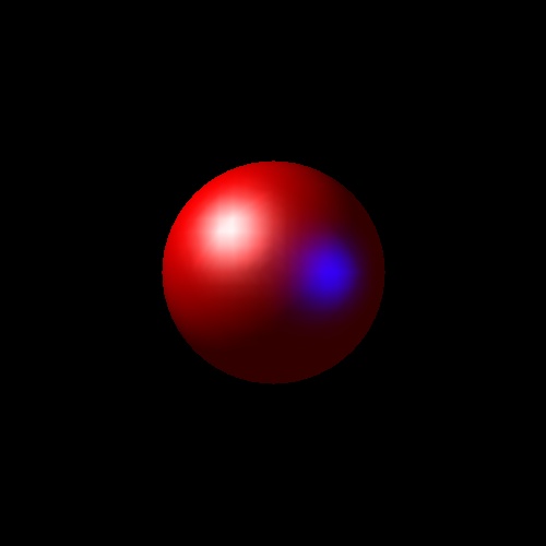
Figure 9 demonstrates Gouraud shading on a sphere using two different colored lights.

Flat Shading

Flat shading is the most basic shading algorithm. The idea behind flat shading is that for each triangle in our solid surface representation, we call the lighting model function once with the average vertex position and average normal and then use the resulting color for every pixel we rasterize on the triangle. We can write the following pseudocode for the algorithm:

where Raster_Flat_Colored_Triangle would be the same as Raster_Colored_Triangle, except it would color each pixel using $colo{r}_{avg}$ rather than interpolated color values. Note that this algorithm is not complete; we would want to incorporate depth buffering and backface culling for full efficiency. These two topics are discussed in the next section.

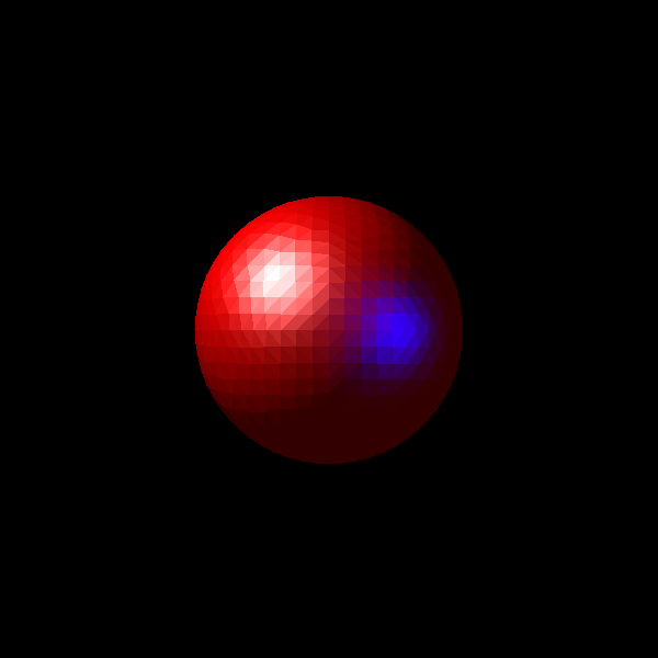
Compare the following sphere image in Figure 10 with the the sphere image in Figure 9. The one in Figure 10 was rendered using flat shading while the one in Figure 9 was rendered using Gouraud shading. We see that flat shading resulted in a more blocky and unrealistic looking coloring. However, because flat shading is so simplistic, it performs much faster than Gouraud shading. As a result, flat shading provides a faster alternative to Gouraud shading if detail is not a priority.

Phong Shading

Phong shading is named after Bui Tuong Phong, who published the technique in 1973. It is the most complex of the three shading algorithms and produces what many consider the “best” shading effect.

Instead of interpolating the colors across the vertices like in Gouraud shading, Phong shading interpolates the world coordinates and normals of the vertices across the triangle. Then, during the rasterization process, for each pixel we rasterize, we call the lighting model with the world coordinates and normal corresponding to the pixel and rasterize the pixel with the resulting color. This technique produces a smoother shading effect than Gouraud shading, but at the cost of more computation; hence, Phong shading does not completely overshadow Gouraud shading. Since Phong shading computes the lighting per pixel, it is often referred to as per pixel lighting.

We can write the following pseudocode for the algorithm:

Note that $v_a$, $v_b$, and $v_c$ in line 19 are in world coordinates.

Compare the following sphere image in Figure 11 with the the sphere image in Figure 9. The one in Figure 11 was rendered using Phong shading while the one in Figure 9 was rendered using Gouraud shading. If you concentrate on the specular highlights, then you can see that the highlights in the image rendered with Gouraud shading are a bit pixelated while the highlights in the image below are much smoother looking.

Note that this algorithm is not complete; we would want to incorporate depth buffering and backface culling for full efficiency. These two topics are discussed in the next section.

Section 4: Discarding Unnecessary Output

Because the shading algorithms can be computationally intensive, we do not want to waste computation time trying to render anything that we do not need. For instance, if a triangle $T_1$ were behind another triangle $T_2$ that is closer to the camera, then we should not waste computation time rendering $T_1$ when $T_2$ will be blocking it from our view. We handle these kinds of cases with depth buffering and backface culling.

Depth Buffering

Depth buffering allows us to determine whether a point that we are trying to rasterize is behind another point and thus should not be rasterized. We do depth buffering in the following manner:

• Create a “buffer grid” with the same dimensions as our raster grid.
• Initialize every element of the grid to a very high value (e.g. the maximum double value).
• For each point $p$ that we consider rasterizing at $\left(x,y\right)$ in our raster grid, check whether the z-position $z$ of the point in NDC is less than the value stored at $\left(x,y\right)$ in the buffer. If it is, then we set that value at $\left(x,y\right)$ in our buffer to $z$ and render the point $p$. Else, we do not render $p$ or change the buffer.

Basically, our “buffer grid” keeps track of the relative distance in NDC between the camera and the closest point to the camera at each square of our raster grid. This allows us to easily check whether a point we are trying to render is behind another point.

Backface Culling

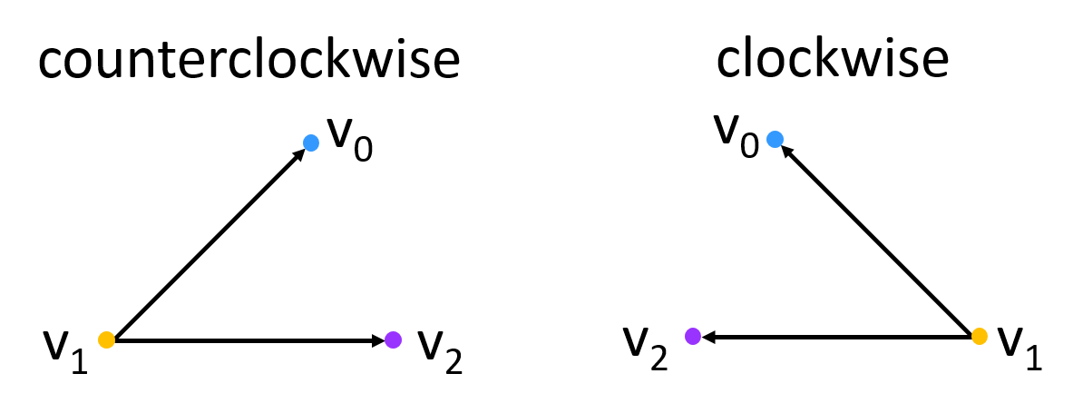
In computer graphics, we use the convention that triangles whose vertices are listed in counterclockwise order face toward the camera. And triangles whose vertices are listed in clockwise order face away from the camera. For an example of a case where a triangle faces away from the camera, just consider all the triangles on the backside of the sphere in Figure 11. Half of the sphere surface is facing towards us, and half of it is facing away from us.

If a triangle with vertices $v_0,v_1,v_2$ were facing toward the camera, then the cross product of vectors $\left(v_2-v_1\right)$ and $\left(v_0-v_1\right)$ in NDC results in a vector whose $z$ component is positive in NDC. On the other hand, the same calculation on a back-facing triangle would result in a vector with a negative $z$ component in NDC. Consider Figure 12:

Recall that NDC has an inverted z-axis. Keeping this in mind, we can use the right-hand rule to verify that $\left(v_2-v_1\right)\times \left(v_0-v_1\right)$ has a positive $z$ component in NDC for front-facing triangles and a negative $z$ component for back-facing triangles.

Section 5: Full Gouraud Shading Algorithm

We can now incorporate depth buffering and backface culling into our Gouraud shading algorithm. To do so, we only need to change Algorithm 5 in the Gouraud Shading section. Algorithm 4 from the same section remains the same.