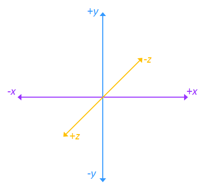
Figure 1: World space coordiante axes.
Assignment 1 Lecture Notes
The following will act as lecture notes to help you review the material from lecture for the assignment. You can click on the links below to get directed to the appropriate section.
Section 1: Geometric Transformations
Geometric transformations are ubiquitous in computer graphics. The three main geometric transformations that we use are translation, rotation, and scaling. We find it convenient to implement these transformations as matrix operations. This requires us to work with homogeneous coordinates instead of the usual Cartesian coordinates. For a given point in three dimensional space with Cartesian coordinates , we express it in homogeneous coordinates where is known as the homogeneous component. The following shows the general mapping between Cartesian and homogeneous coordinates for three dimensions:
Homogeneous coordinates allow us to represent geometric transformations in matrix form and their operation on points as simple matrix multiplications. Consider the translation operation. In Cartesian coordinates, the translation of a point at position by a vector shifts it to the new position . We can implement this operation as a matrix multiplication by expressing translation in the following matrix form:
and then multiplying the translation matrix with the homogeneous representation of (letting the component equal 1):
As you can see, our result is the homogeneous representation of the new position with the homogeneous component equal to 1.
Rotation and scaling are achieved similarly. The following matirx is the rotation matrix for rotating about an axis in the direction of the unit vector counterclockwise by an angle :
And the following is the scaling matrix for scaling the coordinates of a point by the vector :
And of course, consecutive transformations can be combined into a single matrix representation. For instance, a scaling by vector followed by a translation by vector of a point at can be given as:
Section 2: World Space to Camera Space
Rendering in computer graphics is all about turning a mathematical model of a scene into an image that we can perceive. We refer to the coordinate space containing the points in our scene as the world space. Figure 1 shows the world space axes. Note that the coordinate axes here differ slightly from the traditional 3D axes in mathematics.
Figure 1: World space coordiante axes.
In order to obtain an image of our scene, we need to specify in world space a viewing location and angle from which we look. Consider Figure 2:
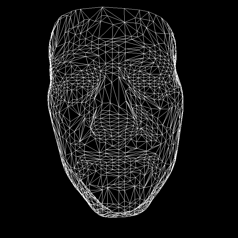
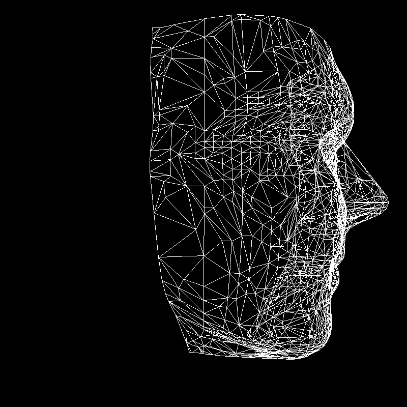
Figure 2: A wireframe of a face mesh shown from two different viewpoints.
Let the face mesh shown above be centered at the origin of our world space. Our default viewing location is at the origin and our default viewing angle causes us to look straight ahead in the direction of the negative z-axis. We can consider the image on the left as what we would see after moving or translating to some point along the positive z-axis. The image on the right would be what we see after we first rotate ourselves 90 degrees clockwise about the y-axis and then translate to some point along the negative x-axis.
We refer to our viewing location as the camera position and the viewing angle as the camera orientation - i.e. we consider ourselves to be looking at our scene through a camera. From the above example, we can see that it would be intuitive to specify the camera position with a translation vector and the camera orientation with a rotation axis and angle. Hence, whenever we set up a camera, we always rotate it by a specified angle about a specified axis and then translate it to a specified point.
Denote the translation matrix for the camera position as and the rotation matrix for the camera orientation as . Then let be the matrix describing the overall transformation for the camera. Suppose that after we set up the camera, we want to transform the entire world space into a new space with the camera at the origin and in its default orientation. This new space, which we call the camera space, provides some advantages that we will see in the next section. We can intuitively see that in order to go from world space to camera space, we apply the inverse camera transform, , to every point in world space.
Note that the terms eye position, eye orientation, and eye space are sometimes used instead of their respective camera counterparts. Their usage is just a terminology preference, and there are no differences in the meanings. For this class, we will use the camera terms, but we should also be aware that the eye terms exist.
Section 3: Perspective Projection
When we look at a scene in real life with our eyes, objects further in the distance appear smaller than objects close by. The technical term for this effect is perspective. We want to reproduce this effect when we render scenes in computer graphics to make them look realistic. We can do so with the following process. We first surround our scene in camera space with a sideways frustum, which, when upright, is the bottom half of a square pyramid that has been cut in two along a plane perpendicular to the axis connecting the tip of the pyramid and the center of the square base. We map every point in the sideways frustum to a cube with what is called a perspective projection. A visual of the mapping is provided in Figure 3.
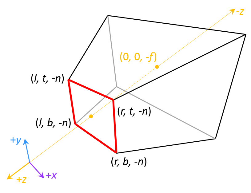
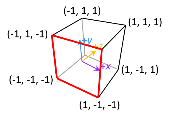
Figure 3: The frustum in camera space is mapped to a cube by what is called a
perspective projection. The smaller base of the frustrum (outlined in red) is mapped
directly to the front face of the cube (also outlined in red). The rest of the frustum has to
be shrunken down to form the rest of the cube.
The key idea here is that all of the frustum beyond the smaller base (outlined in red in Figure 3) must shrink in order to form the cube. For the frustum to shrink, points in the frustum must be clustered closer together. The further away a set of points is from the smaller base of the frustum, the closer together the points are clustered. This clustering causes the objects that those points form to shrink and get rendered smaller than their actual size, creating the desired perspective effect.
The cube resides in its own coordinate system known as normalized device coordinates or NDC for short. Note that this coordinate system has an inverted z-axis. This is due to convention.
We specify a perspective projection with parameters for the dimensions of the frustum. stand for left, right, top, bottom and provide the dimensions for the smaller base of the frustum, which we will now call the near plane or projection plane. stands for near and specifies in camera space the magnitude of the negative z-coordinate of where the frustum begins. stands for far and specifies in camera space the magnitude of the negative z-coordinate of where the frustum ends.
We will now do a quick derivation of the perspective projection matrix, which transforms points from camera space into NDC given and . We first look at just the and coordinate mappings. Let be the position of a point in our camera space and be the same position in homogeneous NDC.
Recall that the projection plane of the frustum is mapped directly to the front of the cube. Since the and mappings do not need to take depth (i.e. the z-coordinate) into account, we can consider them as first mapping pairs of onto the projection plane, and then mapping the projection plane onto a cube face. Let and be the corresponding and coordinates on the projection plane. Figure 4 shows a visual of . A similar idea is used for .
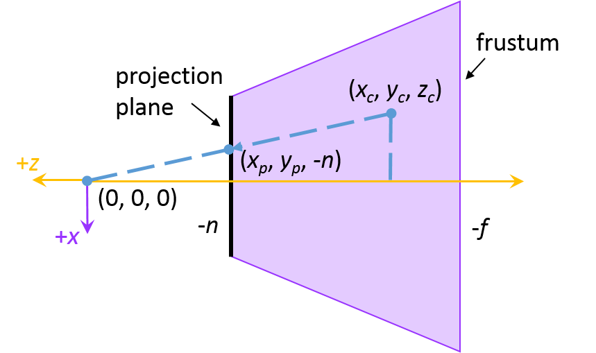
Figure 4: The perspective projection mapping for the
and
coordinates from camera space to NDC can be thought of as first mapping the coordinates
onto the projection plane and then mapping the projection plane onto a cube face.
The values of and are determined using ratios of similar triangles:
This gives us and . We then get the direct mappings for and by solving the linear equations for and .
where and are constants that we need to solve for. Solving the above equations and substituting in and yields:
Recall that we are working in homogeneous coordinates, hence our perspective projection matrix is going to need to accommodate for the component. What we can do is take advantage of the fact that both and have a division by and make while making and equal to just their respective numerator portions from the above equations. We then have:
For the third row, we use the fact that does not depend on or to write:
for coefficients and . We then have:
Using the mappings and and doing some algebra gives us and and:
as the perspective projection matrix. This is the transformation matrix we use to transform a point in camera space to the homogeneous NDC. To go from homogeneous NDC to Cartesian NDC, we would divide our and terms by .
Note that sometimes the frustum we specify does not capture our entire scene, in which case, the points that were outside our frustum in camera space are mapped to the outside of the cube in NDC. These points are outside our field of view and should not be considered for rendering. Hence, when we later render what we see, we need to check for whether a given point is outside the cube. If it is, then we do not render the point.
We render our 3D scene by mapping all of its points in NDC onto a 2D grid of square pixels that we then display onto the screen. This process is known as rasterization. For each point in NDC, we map its and coordinates to a row (r) and column (c) ordered pair with and . We then fill the pixel at to show the point in the display. The coordinate of our point is used for depth buffering and backface culling, which we will cover on the next assignment. Sometimes, the coordinates for the grid are referred to as screen coordinates.
In this section, we will talk specifically about line rasterization. In order to rasterize a line with a grid of pixels, we must decide which squares around the line form the best approximation of the line when filled. Figure 5 shows a visual of this in action:
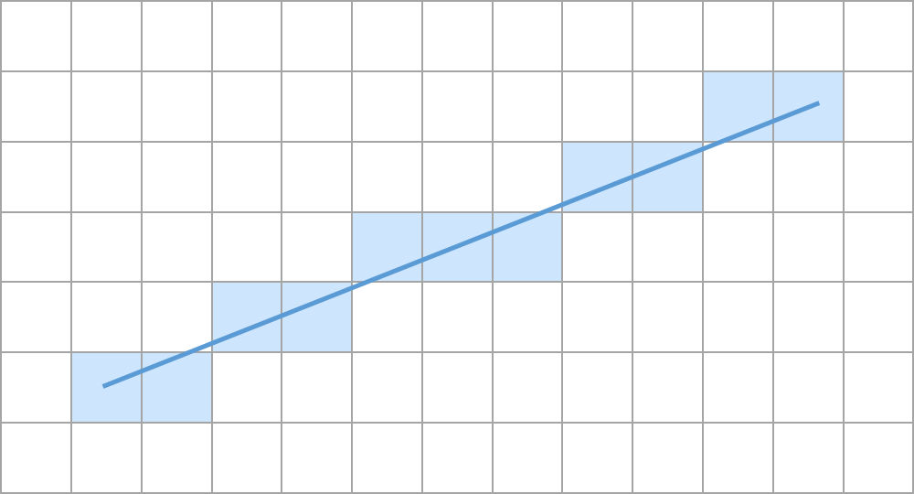
Figure 5: Rasterizing a line by approximating it using a grid of pixels.
The fastest and simplest algorithm that does this is Bresenham’s line algorithm.
The basic Bresenham’s algorithm only works in one octant of the 2D coordinate plane, but it can be generalized to account for the other octants. The generalization will be left as an exercise in the assignment. For now, we will restrict ourselves to discussing the algorithm in just the first octant - i.e. line slopes are in the range . Since it is more natural to talk about lines in terms of and , we are going to use to refer to the column values and to refer to the row values of our grid.
So we wish to connect two points and in the first octant of our grid with an approximation of a line. Let us decide to iterate over the x-coordinate. Then during our routine, if we had just filled in the pixel for some integral point for and , then the next pixel we fill in will have to be either at or . We must decide which one of these points results in a better approximation of the line.
Let denote the error between of the integral point and the true in the actual line. The true is then equal to . When moving from to , we increase the true by the slope . Consider the case where is less than the midpoint of and - i.e. . If that is the case, then the next point in our line is closer to the pixel at than the pixel at . Hence, the next pixel that we would want to fill is at . We would then update as . However, if , then the next pixel should be at and we would update as . This leads us to the following algorithm:
We can optimize this algorithm by eliminating any dependence on floating point values. Consider the following manipulations on the inequality:
Let . Our inequality becomes:
And we can express and as and respectively. This leads us to an algorithm with operations that involve only integers:
Note how the only operations in this algorithm are simple (and fast) arithmetic operations between integers. In addition, the multiplication by 2 can be implemented using a bit-shift. Hence, we end up with a fast and efficient line drawing algorithm for the first octant. The generalization to all octants will also maintain the simplicity and efficiency. As we mentioned before, the generalization will be left as an exercise in the assignment.
Written by Kevin (Kevli) Li (Class of 2016).
Links: Home Assignments Contacts Policies Resources