LEAD Computer Science - Lab 4

Due: Monday, July 23 at 8pm

Please complete all parts of this lab in a file called lab4.py. When you are finished, submit the file on csman for Lab 4.

This lab will deal with recursion. You'll some non-graphical and then some graphical functions to help you understand how recursion works.

Basic exercises involving recursion

Write the following functions using recursion instead of e.g. a loop. Make sure you identify what the base case or cases are and handle them first (a base case is one that can be solved without using recursion). Therefore, your functions will all contain an if/else statement at the beginning. If you're unsure about how recursion works, you should talk to the instructors before attempting the problems, or you might end up spending a lot of time being frustrated! Recursion is often tricky for new programmers, so don't despair; like riding a bike, once you get it, you never forget it. Also, once you "get" recursion, your mind will be expanded and you'll feel enlightened :-)

As usual, don't forget to write docstrings for all of your functions.

Write a function called countdown which takes one argument (a positive integer n), and prints each number from n down to (but not including) zero, with one number per line. For instance:
```
>>> countdown(5)
5
4
3
2
1
```
(This is really easy to do with a for or while loop, but don't do it that way! The solution using recursion is also very short.)
Write a recursive function called fibonacci to compute the nth term in the fibonacci sequence. The fibonacci sequence is a sequence of numbers that starts with 0 and 1, and every subsequent number is the sum of the previous two numbers in the sequence (which sounds very recursive... hmmm...). The sequence looks like this:
```
fibonacci sequence: 0, 1, 1, 2, 3, 5, 8, 13, 21, 34, 55, ...
```
The 0th element of this sequence is 0, the 1th element is 1, and so forth. So the function should work like this:
```
>>> fibonacci(0)
0
>>> fibonacci(1)
1
>>> fibonacci(2)
1
>>> fibonacci(3)
2
>>> fibonacci(4)
3
>>> fibonacci(5)
5
# etc.
```
The mathematical definition of the fibonacci function is:
```
fibonacci(0) = 0
fibonacci(1) = 1
fibonacci(n) = fibonacci(n - 1) + fibonacci(n - 2)  [n > 1]
```
This suggests that the fibonacci function you define in python will have two recursive calls, not one.

Try some larger numbers (say, fibonacci(40)). Does it take a long time to execute? It turns out that the most straightforward way to write a recursive function to compute fibonacci numbers is extremely inefficient (that's OK here; we want you to do it that way). There is a whole field of computer science called computational complexity that deals with how to compute the efficiency of functions.
If you want to compute one number raised to the power of another, you can use the ** operator. For instance, 3 to the 4th power is written as 3**4, which is 81. Let's pretend that this operator didn't exist in Python. Write a recursive function called power that computes one number raised to the power of another. Examples:
```
>>> power(10, 0)
1
>>> power(10, 1)
10
>>> power(10, 3)
1000
>>> power(3, 4)
81
```
Use assertions (see the debugging lecture) to make sure that the first argument is at least 1, and the second argument is at least 0.

Again, this can be easily solved with a for or while loop, but don't do it that way! Think about what the base case should be. Think about how you could decompose a power computation in terms of a smaller power computation. Which argument will have to change between recursive calls? Which one can stay the same?

Recursion and graphics

Now we're going to combine what you know about recursion with turtle graphics to create interesing pictures.

Some of the exercises require code similar to what you've implemented in lab 3. You should feel free to copy that code into this lab, but get rid of all unnecessary features in the code. For instance, if you don't need to draw filled squares, get rid of the code involving filling. If you don't need to draw colored squares, get rid of the code involving color.

As usual, don't forget to write docstrings for all of your functions.

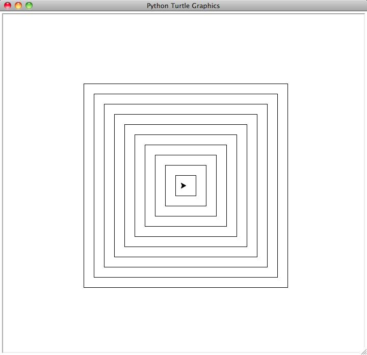
Write a function called draw_nested_squares_1 which takes three arguments: a positive integer n which represents the number of nested squares to draw, a number called size which represents the size of the sides of the first square drawn (in pixels), and a number called d (for "decrement") which represents how much to decrease the size of the squares each time you draw one. The squares should all be centered on the initial location of the turtle, and the turtle should return to that location after drawing each square. Do not use a for or a while loop in this problem; instead, use recursion as follows. If n is zero or the size is less than zero, just return without drawing anything. Otherwise, draw a square and recursively call the function with smaller n and d values.

For instance, the function call draw_nested_squares_1(10, 400, 40) will give an image that looks like this:
Write a function called draw_nested_squares_2 which takes three arguments: a positive integer n which represents the number of nested squares to draw, a number called size which represents the size of the sides of the first square drawn (in pixels), and a number called m (for "multiplier") which represents how much to multiply the size of the squares each time you draw one. m should be in the range (0.0, 1.0) so that the squares will shrink each time. Use an assert statement to check this. The squares should all be centered on the initial location of the turtle, and the turtle should return to that location after drawing each square. Again, do not use a for or a while loop in this problem; instead, use recursion as in the previous problem.

For instance, the function call draw_nested_squares_2(20, 400, 0.9) will give an image that looks like this:

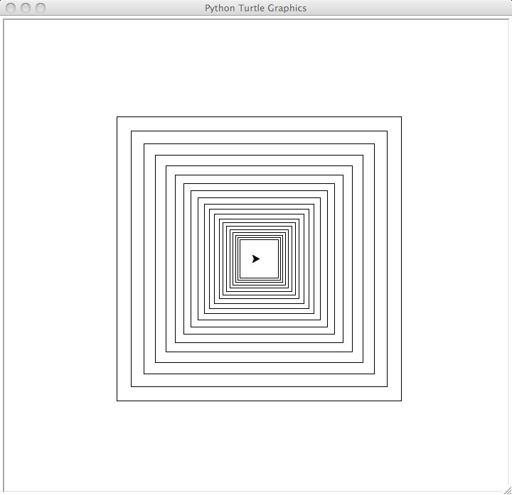
Notice the difference relative to the previous picture; this one looks like you're looking down a tunnel.
Now for our final nested squares example -- the best of all! Write a function called draw_nested_squares_3 which takes four arguments: the number of squares and size as before, the multiplier as in the last problem, and a positive integer which represents the number of degrees to rotate each square relative to the previous square drawn. Again, use recursion has you have been doing previously. Again, use assert statements to check that the multiplier is in the right range and that the rotation is between 0 and 360 degrees.

For instance, the function call draw_nested_squares_3(20, 400, 0.9, 10) will give an image that looks like this:

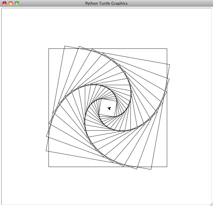
Cool, huh? Experiment with smaller and larger multipliers, and different numbers of degree rotations.

Extra credit: More complex graphics

These examples are considerably more difficult. If you have time, try them out, but you're not responsible for them.

The Hilbert curve

Before you start writing functions to draw more complex pictures, download this file and run it from the terminal as follows (the % is the prompt; don't type that):

% python hilbert.py 1
% python hilbert.py 2
% python hilbert.py 3
% python hilbert.py 4
% python hilbert.py 5
% python hilbert.py 6

Even though these images may look complex, they are generated using a very simple function that is less than 20 lines long. Recursion is what makes this possible. Look at the code and try to figure out how it works. (Technically, this kind of image is called a space-filling curve because the line being traced out is a one-dimensional line which covers a two-dimensional space.) These images are called Hilbert curves after the famous mathematician David Hilbert who discovered them. Hilbert curves are also considered to be fractals, which is a generic name for geometric objects that exhibit a high degree of self-similarity. If you look closely at a Hilbert curve of degree 6 (generated by python hilbert.py 6), you'll see 4 Hilbert curves of degree 5, and each of those will contain 4 Hilbert curves of degree 4, etc. Fractals are very intriguing geometrical objects both visually and conceptually. They are like a visual representation of recursion.

This section (the Hilbert curve) was just for illustration purposes; there is nothing to hand in.

The Koch snowflake

Now that you've seen what a fractal looks like, let's make one! First, consider a straight line:

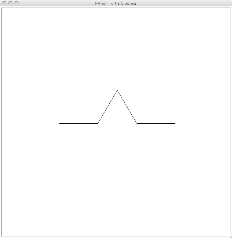
Imagine dividing that line up into three equal parts. Remove the middle part, and replace it by two more parts of the same size, connected to the two original parts that remain. The two new parts are at a 60 degree angle to the original line. The result looks like this:

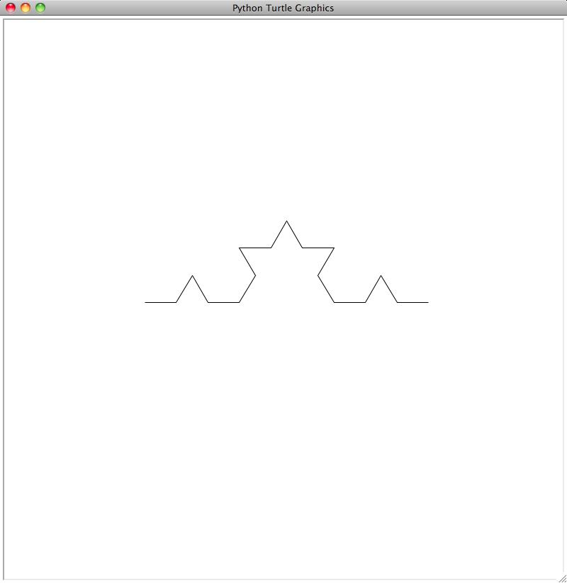
Here is where it becomes fun. The figure we just showed you has four lines in it. Take each of those four lines, and transform it like you did the first original line. The result is this:

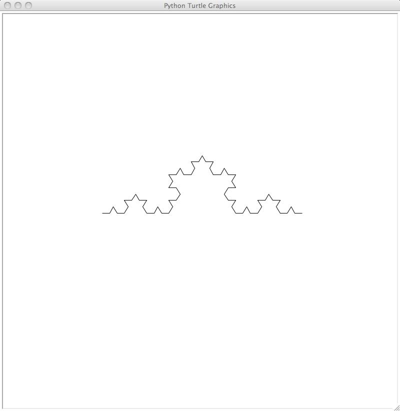
Note how the original line after two transformations of this kind is becoming more and more bumpy. We can keep repeating this transformation for every line in the new figure, leading to this:

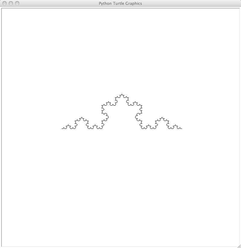
One more transformation of this kind gives us this figure:

And one more transformation gives this:

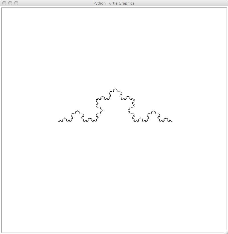
We could continue like this, but you get the point. As the transformation is performed over and over (we say that it is iterated), the original straight line gets bumpier and bumpier. Also, every time you do a transformation, the total length of all the lines in the figure increases by a factor of 4/3.

Now for one last trick. Instead of starting with a single line, what if we started with an equilateral triangle (with angles of 60 degrees)? Then we would generate this shape after a few transformations:

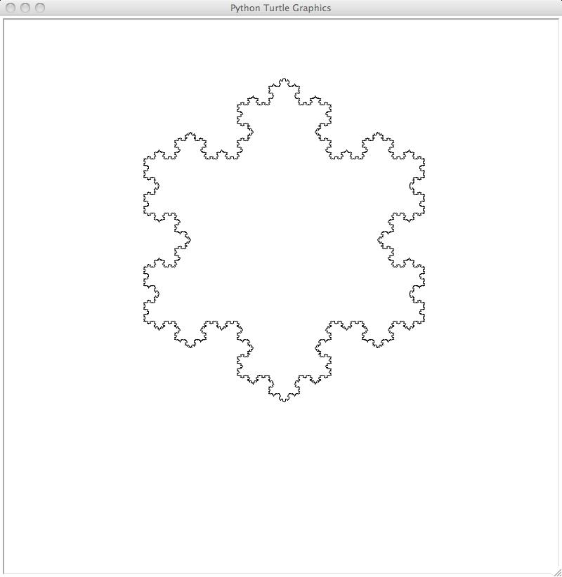
This shape is called the "Koch snowflake", after the Swedish mathematician Helge von Koch, who discovered it.

OK, now here's how you draw it. First, write a function called koch_side which will draw one side of a Koch snowflake (like the images above, except for the last one). This function takes two arguments: the length of the original side and the number of times to divide it up according to the algorithm described above. The images you've seen above (except for the last one), were generated from these calls to koch_side on a window of size 800x800 pixels:

koch_side(400.0, 0)  # straight line
koch_side(400.0, 1)
koch_side(400.0, 2)
koch_side(400.0, 3)
koch_side(400.0, 4)
koch_side(400.0, 5)

You may find this function to be a bit tricky to write, even though it's only a few lines long. Use recursion, and use the case where the second argument is 0 as your base case (in that case, just draw a straight line). Before implementing the recursion, you should make sure you can draw the first two images shown above. Then replace the straight line drawing parts with recursive calls to get the full function. What part of the function call has to decrease with each recursive call? By how much?

Once you've figured out how to draw the sides of a Koch snowflake, the entire image is easy to draw: just draw three sides, each rotated 120 degrees relative to the previous side. If you do it right, you now have a drawing of a Koch snowflake!

The Sierpinski triangle

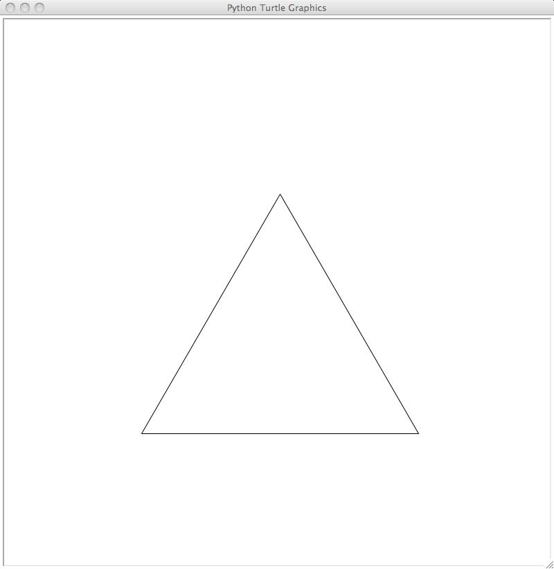
Now that we've drawn one fractal shape, let's draw another. The Sierpinski triangle is a fractal shape made as follows. First, draw a triangle oriented with the base at the bottom of the triangle, like this:

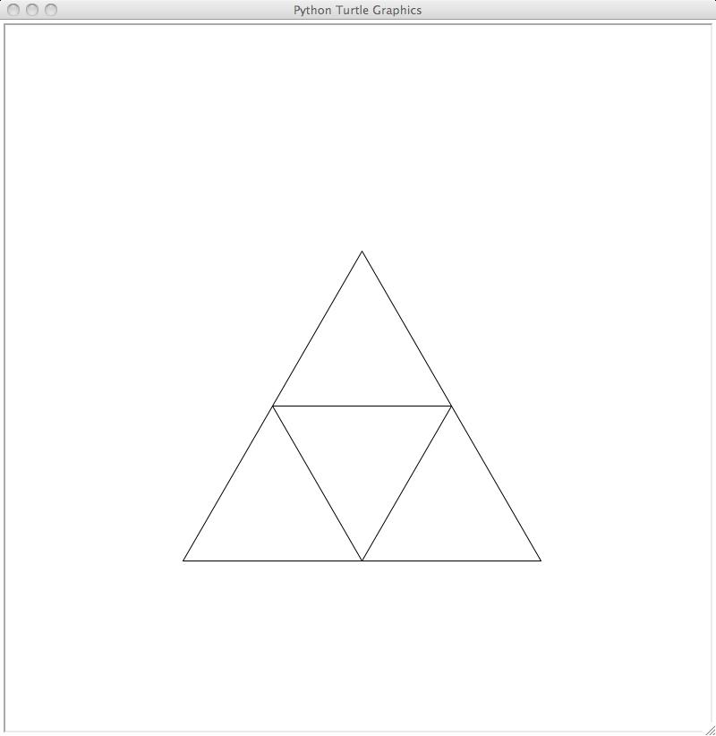
We'll call this orientation of a triangle an "upward-facing triangle", and the opposite orientation a "downward-facing triangle". Now draw a downward-facing triangle of half the size, starting in the middle of one of the edges of the original triangle. This gives this image:

Notice that this image has three small upward-facing triangles. What if we drew downward-facing triangles in the middle of each of them? The result would be this:

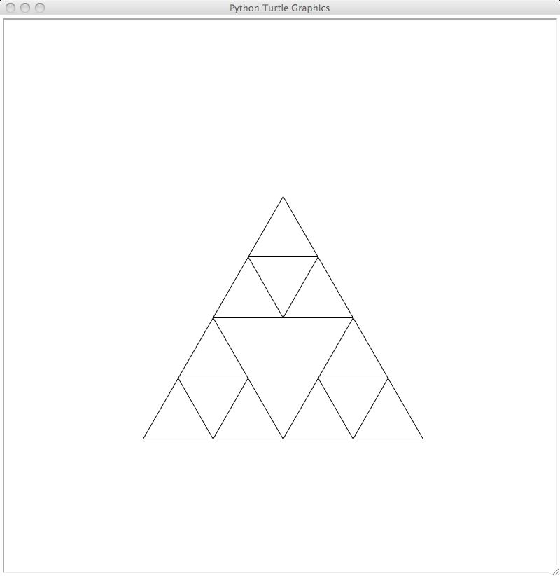
Now we have nine small upward-facing triangles. Again, draw downward-facing triangles in the middle of each of them, to get this:

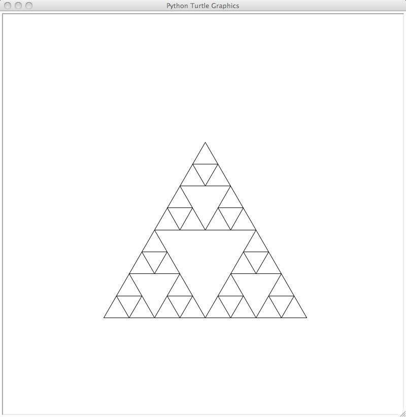
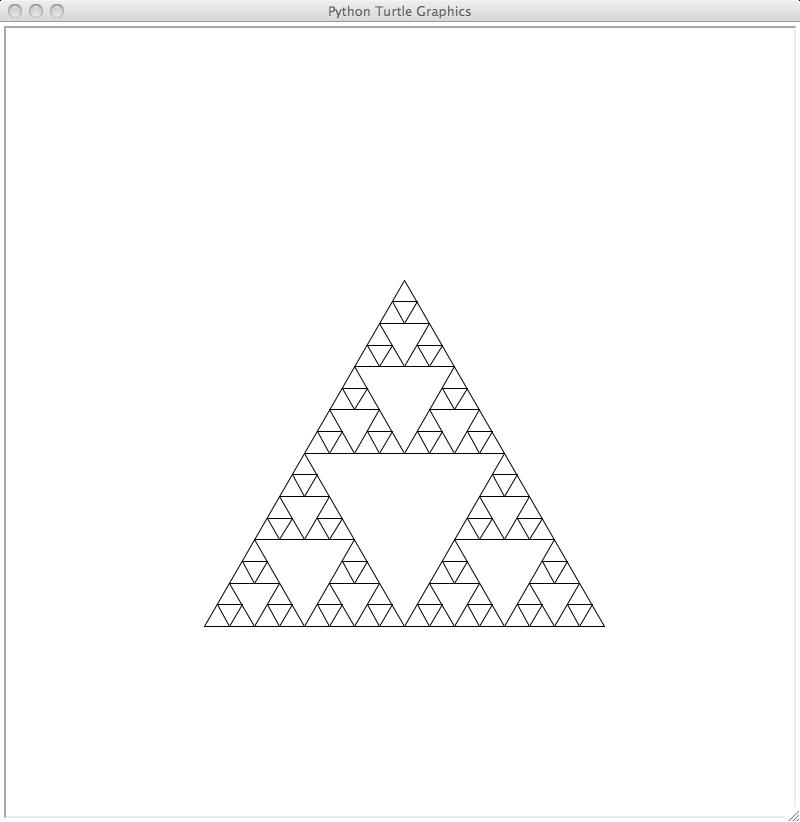
Repeat this process a few more times, to get these images:

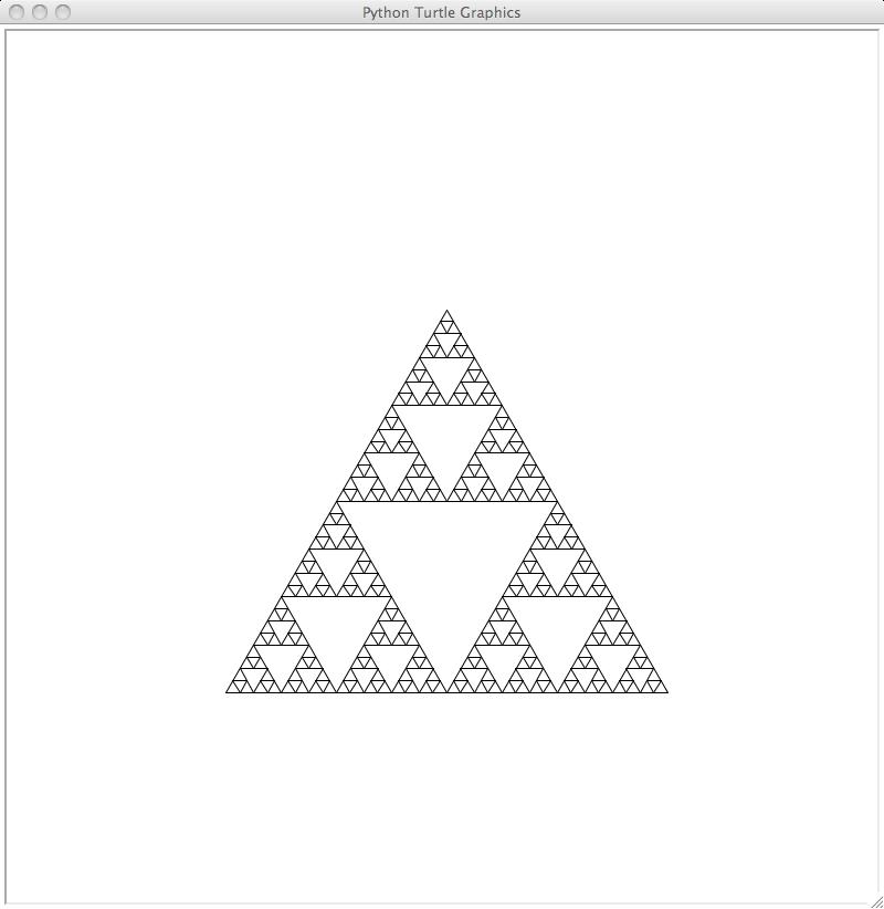
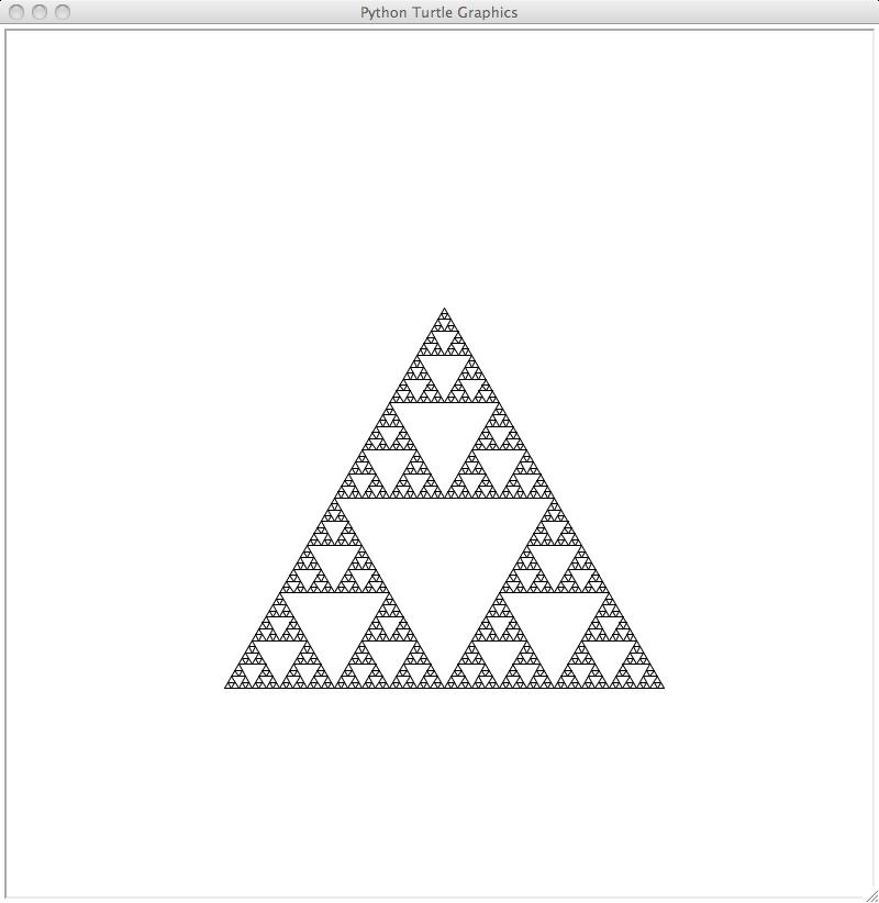
This fractal shape is the Sierpinski triangle. Notice that apart from the first upward-facing triangle, all you're actually drawing are downward-facing triangles.

Here's how to draw the Sierpinski triangle:

First, write functions to draw upward-facing triangles of a particular side length (equilateral triangles) and downward-facing triangles of a particular side length.
Write a function called sierpinski which takes two arguments: the size of a side of the Sierpinski triangle (in pixels) and the number of levels of iteration (where level 0 is just an upward-facing triangle, level 1 includes one downward-facing triangle, level 2 contains smaller downward-facing triangles, and so on like in the pictures above). This will draw the outermost upward-facing triangle of a Sierpinski triangle, and if the level is greater than 0, it will call the function sp_helper to complete the drawing.
Write a function called sp_helper which takes the same two arguments as sierpinski. The level argument should be at least 1 (you can use an assert to check for this). This will draw the largest downward-facing triangle for the Sierpinski triangle, and if the level is greater than 1, it will call itself recursively with the size halved and the level decreased by 1. It will have to call itself recursively a total of three times to completely fill up the Sierpinski triangle. Each time the turtle will need to be at a different location, so make sure you move it after each recursive call.

Hint: All the real work of this drawing happens in the sp_helper function. It's very easy to make mistakes here, but one way to keep things simple is to make sure that every time you draw a downward-facing triangle inside an upward-facing triangle, you return to the lower-left corner of the upward-facing triangle.

Speeding up your drawings

When drawing fractals, your program often has to draw a very large number of line segments. The normal drawing speed of the turtle graphics module is much too slow to do this in a reasonable amount of time. You can set the speed to the highest value by setting speed(0), but even that isn't enough. The way to get the absolute maximum drawing speed is to turn tracing of the image by the turtle completely off. Before you start a drawing, you can include this code:

tracer(0)

This will turn tracing off. Then do the drawing, and at the end, include this code:

update()
tracer()

The first line causes the drawing to appear, and the second line turns tracing back on.

You only really need to do this for the drawings in the second part of the lab. You can do it on a function-by-function basis.

You probably also want to hide the turtle using hideturtle() because the turtle is more of a nuisance than a help when drawing fractals (at least when there are a large number of lines to draw).

Submission

Once you have completed this lab, submit lab4.py for Lab 4 on csman.