Assignment 7 Lecture Notes

The following will act as lecture notes to help you review the material from lecture for the assignment. You can click on the links below to get directed to the appropriate section.

• Section 1: Superquadrics
  • 1.1 Inside-Outside Functions
  • 1.2 Definition
  • 1.3 Normals
  • 1.4 Examples
  • 1.5 Transforming Implicit Functions
• Section 2: Raytracing
  • 2.1 Intersections
    • 2.1.1 Newton’s Method
    • 2.1.2 Initial Guess
    • 2.1.3 Stopping Conditions
  • 2.2 The Screen Plane
  • 2.3 Sending Out Rays
  • 2.4 Lighting Models and Shadows

Section 1: Superquadrics

Superquadrics are a family of inside-outside functions (defined below) which allow us to generate a variety of implicit three-dimensional shapes that we can easily compute normals and gradients for; perfect for a simply raytracing program to work with.

1.1 Inside-Outside Functions

In order to define the shapes we’ll be ray tracing, we use an inside-outside function, defined to be some $f:{ℝ}^3\to ℝ$ such that

$$f\left(x,y,z\right)\left\{\begin{array}{cc}<0\hfill & \text{inside the object}\hfill \\ =0\hfill & \text{on the object’s surface}\hfill \\ >0\hfill & \text{outside the object}\hfill \end{array}\right.$$

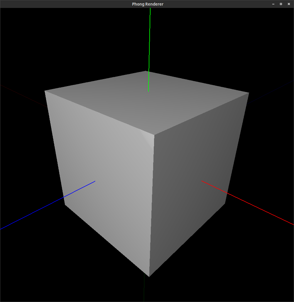
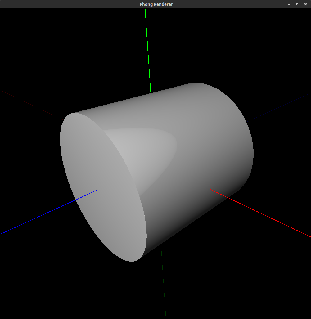
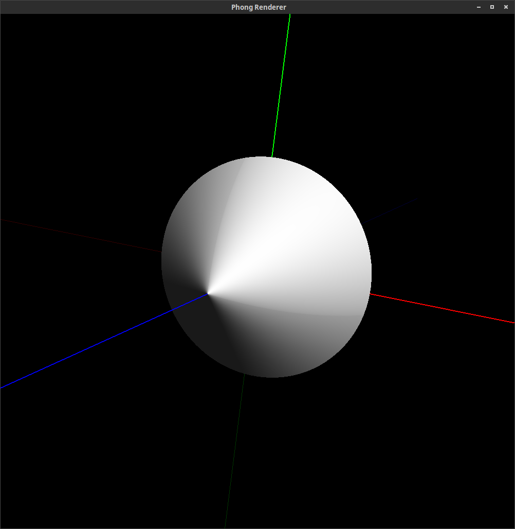
Many common solids can be defined this way, such as the unit cube, unit sphere, octahedron, unit cylinder, and double cone: $$\begin{array}{llll}\hfill \text{cube}\left(x,y,z\right)& =max\left(\left|x\right|,\left|y\right|,\left|z\right|\right)-1& \hfill & \\ \hfill \text{sphere}\left(x,y,z\right)& =x^2+y^2+z^2-1& \hfill & \\ \hfill \text{octahedron}\left(x,y,z\right)& =\left|x\right|+\left|y\right|+\left|z\right|-1& \hfill & \\ \hfill \text{cylinder}\left(x,y,z\right)& =max\left(x^2+y^2,z^2\right)-1& \hfill & \\ \hfill \text{cone}\left(x,y,z\right)& =\sqrt{x^2+y^2}+\left|z\right|-1& \hfill & \end{array}$$

One can see that by setting the left-hand side of side of these equations to 0, we get an implicit definition for each of these shapes.

1.2 Definition

Instead of having to use a variety of different functions for different shapes however, we introduce superquadrics, which themeselves are a three-dimensional generalization of Lamé curves (also known as Piet Hein’s “superellipses”). The general superquadric function can then be defined to mimic the surfaces described above, amongst others. It is even possible to extend the math to create toroids, however, we limit the scope to dealing solely with ellipsoides, defined by a longitudinal shape parameter $e$ and latitudinal parameter $n$. Thus, we get the general inside-outside function of superquadrics as:

$$S\left(x,y,z,e,n\right)={\left({\left(x^2\right)}^{\frac{1}{e}}+{\left(y^2\right)}^{\frac{1}{e}}\right)}^{\frac{e}{n}}+{\left(z^2\right)}^{\frac{1}{n}}-1$$

Looking at the general form, we can verify that when $e=n=1$ this become the same inside-outside function as the unit sphere, and similarly, when $e=n=2$, we have an octahedron. Keep in mind that when computing the result of this function, the squaring of the $x$, $y$ and $z$ values must occur prior to the other exponentiation since negative coordinates would cause computational errors.

1.3 Normals

With an implicit definition of a particular superquadric, we can also compute the surface normal at a given point $\left(x,y,z\right)$ by computing the gradient of the superquadric function. We therefore have:

1.4 Examples

The following images are rendered images of superquadric surfaces. (They were actually rendered with the command line and rendering tool that you will be using in Assignment 7.) By varying the longitudinal and latitudinal parameters, $e$, and $n$ respectively, we can create the shapes shown below.

1.5 Transforming Implicit Functions

So far, we’ve only considered superquadrics centered at the origin, but in order to make scenes, we want to be able to position our objects arbitrarily. Specifically, given some inside-outside function $f\left(\overrightarrow{x}\right)$, we want to know how to find the resulting function $F\left(\overrightarrow{X}\right)$ which serves an inside-outside function for the same surface under some transformation $O$ that takes $\overrightarrow{x}$ to $\overrightarrow{X}$. As an example, let’s consider the transformation given by $$\overrightarrow{X}=O\left(\overrightarrow{x}\right)=T\left(R\left(S\left(\overrightarrow{x}\right)\right)\right),$$

where $T$, $R$, and $S$ are some translation, rotation, and scaling operations respectively. Then, we have the inverse transformation $O^{-1}$ as $$\overrightarrow{x}=O^{-1}\left(\overrightarrow{X}\right)=S^{-1}\left(R^{-1}\left(T^{-1}\left(\overrightarrow{X}\right)\right)\right)$$

We can then plug this into the relation between our original and transformed inside-outside functions to get that $$F\left(\overrightarrow{X}\right)=f\left(\overrightarrow{x}\right)=f\left(O^{-1}\left(\overrightarrow{X}\right)\right).$$

Thus, in order to calculate the inside-outside function of a transformed superquadric, you must first apply the inverse transformation to the position vector in question, and feed this into the original untransformed function.

Keep in mind that when using this technique to make sure that you are clear on what space you are in when you compute different things. For example, if you had a point $\overrightarrow{x}$ that you want to find the surface normal for on some inside-outside function $f\left(\overrightarrow{x}\right)$ under some transformation $O$, then you should transform $\overrightarrow{x}$ to $\overrightarrow{X}$, compute the normal for $\overrightarrow{X}$ using $f$, then transform the resulting normal back by applying $O$ for normals: don’t forget that transformations work differently for normals than points.

On the same note, if you have a directional vector $\overrightarrow{a}$, perhaps if you parameterized a point to be an origin plus a directional vector, in order to compute an inside-outside function $f$ with transformation $O$ properly, the origin needs to be transformed as stated above with the inverse transformation matrix and $\overrightarrow{a}$ should be transformed with the inverse transformation matrix without translations in order to preserve the correct resulting point that corresponds to adding the two. Alternatively, you could compute the actual point by adding the directional vector to the origin prior to doing any transformation and transform the point as stated above.

Section 2: Raytracing

In order to understand what we mean by “a ray for each pixel,” I find that it helps to imagine putting a wire screen, as you might find on a window, in front of your face. You’d still be able to tell what’s behind it, but your vision would be divided up into a grid. If you then chose a point in each square of the grid and colored the entire square to match that point, then you’d end up with a similar-looking image. If the squares were large, it might look highly “pixelated” like an old videogame, but as you increased their density you’d get a sharper image.

This is essentially how scenes are represented on computer screens: we can’t represent the light from the (by definition) infinite number of points, so we sample them at regular intervals and call it good enough. To ray trace an image, we think about the actual grid of pixels on the monitor as being the wire screen from before, and send a ray out from our camera through a point in each pixel in order to fill it in with a color.

2.1 Intersections

Now that we know how to express the surface of a superquadric and compute its normal vectors, how do we follow light from the camera back to the surface of objects? For simple contours such as planes we can solve for the intersection between a vector and the surface explicitly, but for superquadrics we must use an iterative solver to produce an estimation. One such technique that produces accurate results but is still fairly straightforward is that of Newton’s method.

2.1.1 Newton’s Method

Many of you will recall from calculus that a Taylor series $T\left(g\left(t\right),t_0\right)$ is a method of approximating the function $g\left(t\right)$ around the point $t=t_0$, given by $$g\left(t\right)=g\left(t_0\right)+g^{\prime }\left(t_0\right)\left(t-t_0\right)+\dots$$

If we ignore the higher order terms as they are comparatively small in the neighborhood of $t_0$, then we can say that if $g\left(t\right)=0$, we have $$0=g\left(t_0\right)+g^{\prime }\left(t_0\right)\left(t-t_0\right)\Rightarrow t=t_0-\frac{g\left(t_0\right)}{g^{\prime }\left(t_0\right)}$$

This tells us that if we’re at some point $t_0$ and want to get to another point $t$ where $t$ is a root of $g\left(t\right)$, then we can approximate $t$ using $t_0$, $g\left(t_0\right)$, and $g^{\prime }\left(t_0\right)$.

This can be made into an iterative process by replacing $t$ with $t_{\text{new}}$ and $t_0$ with $t_{\text{old}}$, so that if we start from some initial value of $t_{\text{old}}$, we can compute our next approximation of $t$ as $$t_{\text{new}}=t_{\text{old}}-\frac{g\left(t_{\text{old}}\right)}{g^{\prime }\left(t_{\text{old}}\right)},$$

and then plug this again in as $t_{\text{old}}$ to get another approximation of $t$, and so on and so forth until we hit some “stopping condition.” We label this value as $t_{\text{final}}$, and take it to be that $g\left(t_{\text{final}}\right)\approx 0$. As you may have guessed, we will be using the superquadric function ($S$) and its derivative for $g$ and $g^{\prime }$, since finding the intersection of a vector and a superquadric’s surface is the same as finding where along the vector we will have $\text{S}\left(x,y,z,e,n\right)=0$.

It is of course possible that $g^{\prime }\left(t_0\right)=0$, which would cause divide-by-zero errors at runtime - you should check for this.

2.1.2 Initial Guess

So what do we use as our initial value of $t_{\text{old}}$? A simple way to bound superquadrics is to use a sphere larger than the largest unit superquadric, which is a cube. The radius of the bounding sphere must therefore be $\sqrt{1^2+1^2+1^2}=\sqrt{3}$, which in turn gives us an inside-outside function for it: $$\text{bsphere}\left(\overrightarrow{x}\right)=\overrightarrow{x}\cdot \overrightarrow{x}-3$$

Now, we know we can express a line parallel to the vector $\overrightarrow{a}$ that passes through $\overrightarrow{b}$ as $$\text{ray}\left(t\right)=\overrightarrow{a}t+\overrightarrow{b}$$

Where $t$ varies across $ℝ$. If we let $\overrightarrow{b}$ be the location of our camera, then we can solve for the intersection of a ray exiting the camera and the bounding sphere of a superquadric by solving

This is just a quadratic equation in $t$ with coefficients $a=\overrightarrow{a}\cdot \overrightarrow{a}$, $b=2\left(\overrightarrow{a}\cdot \overrightarrow{b}\right)$, and $c=\overrightarrow{b}\cdot \overrightarrow{b}-3$, so we can solve for $t$: $$t^{\pm }=\frac{-b\pm \sqrt{b^2-4ac}}{2a}$$

Now, there are two things to consider. The first is that our discriminant may be negative, leading to imaginary values of $t$. This corresponds with cases where the ray misses the bounding sphere entirely, so you should check for this and handle it accordingly.

The second is that we have two solutions for $t$, $t^{+}$ and $t^{-}$. The physical interpretation of this fact is intuitive, as a ray may intersect a sphere in at most two locations. If both values of $t$ are positive, then starting point $\overrightarrow{b}$ is outside the sphere and the smaller value $t^{-}$ is on the side of the sphere closer to the camera, and thus closer to the ray’s actual intersection with the superquadric. In this case, your initial guess should be $t^{-}$.

If one value is positive and the other negative, then $\overrightarrow{b}$ is inside the sphere, and the ray may or may not hit the superquadric while traveling away from the eye. In this case, both $t^{-}$ and $t^{+}$ could be tested as initial guesses. If either produces a positive solution for $t$ through the Newton’s method solver, then the trick is to know whether the ray intersects the superquadric on the way in or the way out. If one solution is positive and one is negative, then we know $\overrightarrow{b}$ is inside the superquadric, and the outside surface can’t be seen. If both are positive, however, then we know the ray goes in one side and comes out the other. If both are negative, then the superquadric is entirely behind the camera, and can’t be seen.

As with the Newton’s method solutions in the previous case, we know that if both $t^{+}$ and $t^{-}$ are negative, then the bounding sphere is behind the camera and thus invisible, since the ray has to travel backwards to hit it.

Note that for the assignment, using $t^{-}$ when it is positive should be sufficient for the scenes we provide.

2.1.3 Stopping Conditions

Between floating point math and the inherent approximation made by our Newton’s method solver, we can’t simply iterate until we find a value of $t$ such that $S\left(\overrightarrow{a}t+\overrightarrow{b}\right)=0$. Instead, we can stop when the value of a superquadric’s inside-outside function is close enough to zero. A good approximation of this is when we are within one twentieth or so of a pixel’s width away from the actual surface, but the gist is that $\left|S\left(\overrightarrow{a}t+\overrightarrow{b}\right)\right|$ must be sufficiently close to 0.

However, we can also take advantage of the fact that we know some information about $g^{\prime }\left(t\right)=\overrightarrow{a}\cdot \nabla S\left(\overrightarrow{a}t+\overrightarrow{b}\right).$ As long as we are approaching the superquadric along a ray, the inside-outside function should be positive and decreasing, and thus $g^{\prime }\left(t\right)$ should be negative. If ever it becomes positive, then traveling further along the ray should take us farther away from the superquadric. Thus, if the sign of $g^{\prime }\left(t\right)$ ever changes from $-$ to $+$, we know we’ve missed the superquadric.

Additionally, on the surface of a superquadric we will have $g^{\prime }\left(t\right)=0$, so if this is ever the case we should also check if $g\left(t\right)=0$. If this is satisfied as well, then we know we’re on the superquadric’s surface already, and can just use our current value for $t_{\text{old}}$ without computing $t_{\text{new}}$. On the other hand, if $g^{\prime }\left(t\right)=0$ and $g\left(t\right)$ is nowhere near 0, the math is effectively the same as the sign change case mentioned above.

Above all else, remember that $\overrightarrow{b}$ is the position of the camera, $\overrightarrow{a}$ is the direction the camera is looking, $$\text{ray}\left(t\right)=\overrightarrow{a}t+\overrightarrow{b}$$

describes a ray leaving the camera, $$g\left(t\right)=S\left(\text{ray}\left(t\right)\right)$$

is the function to use in Newton’s method as it tests whether the ray is inside a superquadric, and $$g^{\prime }\left(t\right)=\overrightarrow{a}\cdot \nabla S\left(\text{ray}\left(t\right)\right)$$

is its derivative.

2.2 The Screen Plane

Now that we know what to do, the question is how to do it: how do we express each ray in the form $\overrightarrow{a}t+\overrightarrow{b}$, so that we can use our Newton’s method solver? This is actually just a poorly-disguised exercise in linear algebra.

First, we define the screen to be the front plane of the camera frustum. In this class so far, you’ve likely only dealt with frustums given by their near, far, left, right, top, and bottom components, but our program uses another common representation based on the near and far components, along with the camera’s vertical field-of-view (FOV) and aspect ratio. The FOV is defined to be the angle between the vector from the camera to the horizontal midpoint of the top of the screen and the vector from the camera to the horizontal midpoint of the bottom of the screen, while the aspect ratio is simply the x-resolution divided by the y-resolution.

From this, we can easily calculate the height and width of the front plane of the frustum, assuming that the camera is centered within it. If its distance from the camera (i.e. the near component) is $n$, the FOV is $\theta$, and the height of the plane is $h$, then from basic trigonometry we know that $$\frac{h∕2}{n}=tan\left(\frac{\theta }{2}\right)\iff h=2ntan\left(\frac{\theta }{2}\right),$$

where $\theta$ is the unique angle in an isosceles triangle of height $n$ and base $h$. If the aspect ratio is then $a$, and the width of the plane is $w$, we have $$\frac{w}{h}=a\iff w=ah.$$

Once we have $w$ and $h$, we can divide the plane up into an $x$ by $y$ grid.

2.3 Sending Out Rays

Now we need to find the vector from the camera through each point on the grid, which can easily be done by finding the vector which would translate us from the camera’s position to that point.

We begin by defining three basis vectors, ${\overrightarrow{e}}_1$, ${\overrightarrow{e}}_2$, and ${\overrightarrow{e}}_3$. ${\overrightarrow{e}}_1$ is simply the direction the camera is looking, which is $\left(0,0,-1\right)$ before the camera rotation is applied. We then take ${\overrightarrow{e}}_2$ to be the one pointing directly to the right relative to the camera, which is initially $\left(1,0,0\right)$, and ${\overrightarrow{e}}_3$ to be the one pointing directly upwards relative to the camera, which is initially $\left(0,1,0\right)$.

Adding $n\cdot {\overrightarrow{e}}_1$ to the camera’s position takes us to the exact center of the screen. If we then translated again by $\frac{w}{2}\cdot {\overrightarrow{e}}_2$ we’d be at the midpoint of the right edge of the screen, and then another translation by $\frac{h}{2}\cdot {\overrightarrow{e}}_3$ would take us to the top right corner. From this, it should make sense that adding or subtracting $\frac{w}{x}\cdot {\overrightarrow{e}}_2$ takes us right or left by a pixel, while adding or subtracting $\frac{h}{y}\cdot {\overrightarrow{e}}_3$ takes us up or down by a pixel.

This is really all we need. If we define $x_i$ to be $\left(i-\frac{x}{2}\right)\frac{w}{x}$, with $i$ being an integer in $\left[0,x\right)$, and $y_j$ to be $\left(j-\frac{y}{2}\right)\frac{h}{y}$, with $j$ being an integer in $\left[0,y\right)$, then pixel $\left(i,j\right)$ can be expressed as $\overrightarrow{b}+n{\overrightarrow{e}}_1+x_i{\overrightarrow{e}}_2+y_j{\overrightarrow{e}}_3$, where $\overrightarrow{b}$ is the position of the camera. You can verify that this produces sane results by plugging in $\left(i,j\right)=\left(0,0\right)$, which should take us to the bottom left corner, or $\left(i,j\right)=\left(x,y\right)$, which should take us to the top right. Note that for the purposes of this derivation, I have defined the $y$-axis to be increasing along the upwards direction, which is the opposite of graphics convention.

Now we recall that our rays should be expressed in the form $\overrightarrow{a}t+\overrightarrow{b}$. It doesn’t really matter how long $\overrightarrow{a}$ is, since whatever value of $t$ we solve for will be correct for the given $\overrightarrow{a}$. Thus, we can simply take $\overrightarrow{a}=n{\overrightarrow{e}}_1+x_i{\overrightarrow{e}}_2+y_j{\overrightarrow{e}}_3$, with $t=1$ taking us to a point on the front plane of the frustum.

2.4 Lighting Model and Shadows

As you should have demonstrated in your intersection test from part a, we can find the normal at any point on the surface of a superquadric. Because the Phong model calculates lighting at any point on a surface given the normal, we can easily reuse it here to figure out the color at a ray-superquadric intersection.

However, ray tracing allows us to incorporate further complexities into the Phong model, the simplest of which is shadowing. Let us define an object to be illuminated by a point light as long as the path from the light to the object is unobstructed. At each point we apply the Phong model to, we can check each light to see if it’s obstructed by sending a ray out from the light to the intersection point (or vice-versa) and testing whether it hits any other superquadrics before hitting the one we initially intersected with. If the intersection point is $\overrightarrow{p}$ and the position of the light is $\overrightarrow{l}$, then $\overrightarrow{a}$ is given as $\overrightarrow{a}=\overrightarrow{p}-\overrightarrow{l}$, and when $t=1$ we’ve reached the intersection point. You must do this in your lighting calculations.

Other more advanced capabilities when using raytracing to render images include handling reflections and refractions, but will not be in the scope for this class. You could imagine that given we implemented all these different extensions, the rendered images become very realistic and life-like since we are effectively modelling light as we see it in our physical world.